Image Classification with Tensorflow Keras
Introduction
Hello Everyone!
Today we will be performing image classification with tensorflow and neural networks!
Let’s begin, as always, by loading in our packages and data. We will be using the cats and dogs data.
§1. Load Packages and Obtain Data
import os
import tensorflow as tf
from tensorflow.keras import utils
from tensorflow import keras
# location of data
_URL = 'https://storage.googleapis.com/mledu-datasets/cats_and_dogs_filtered.zip'

# download the data and extract it
path_to_zip = utils.get_file('cats_and_dogs.zip', origin=_URL, extract=True)

# construct paths
PATH = os.path.join(os.path.dirname(path_to_zip), 'cats_and_dogs_filtered')

train_dir = os.path.join(PATH, 'train')
validation_dir = os.path.join(PATH, 'validation')

# parameters for datasets
BATCH_SIZE = 32
IMG_SIZE = (160, 160)

# construct train and validation datasets
train_dataset = utils.image_dataset_from_directory(train_dir,
                                                   shuffle=True,
                                                   batch_size=BATCH_SIZE,
                                                   image_size=IMG_SIZE)

validation_dataset = utils.image_dataset_from_directory(validation_dir,
                                                        shuffle=True,
                                                        batch_size=BATCH_SIZE,
                                                        image_size=IMG_SIZE)

# construct the test dataset by taking every 5th observation out of the validation dataset
val_batches = tf.data.experimental.cardinality(validation_dataset)
test_dataset = validation_dataset.take(val_batches // 5)
validation_dataset = validation_dataset.skip(val_batches // 5)
Downloading data from https://storage.googleapis.com/mledu-datasets/cats_and_dogs_filtered.zip
68608000/68606236 [==============================] - 1s 0us/step
68616192/68606236 [==============================] - 1s 0us/step
Found 2000 files belonging to 2 classes.
Found 1000 files belonging to 2 classes.
# technical code related to rapidly repeating data

AUTOTUNE = tf.data.AUTOTUNE

train_dataset = train_dataset.prefetch(buffer_size=AUTOTUNE)
validation_dataset = validation_dataset.prefetch(buffer_size=AUTOTUNE)
test_dataset = test_dataset.prefetch(buffer_size=AUTOTUNE)
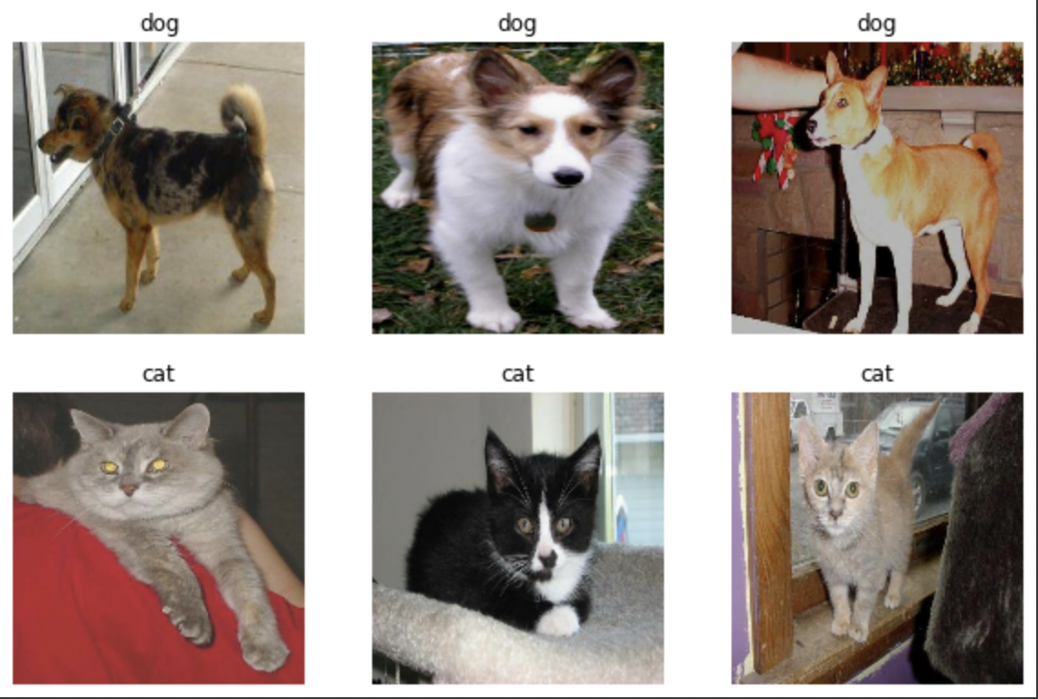
Now that we have our data, let’s visualize it! We’ll be printing out some images and their corresponding labels.
Working with Datasets
Let’s visualize our data, but have the top row be dogs and the bottom row be cats.
def plot_imgs(dataset):
    """plots images in two rows of three; top is one category and bottom is a second

    @param dataset: dataset with images and labels
    @return: 6 images in rows of 2
    """
    #set class names
    class_names = ['cat','dog']

    #empty list for dogs and cats, images + labels
    dogs = []
    cats = []

    #set fig size
    plt.figure(figsize=(10, 10))

    for images, labels in dataset.take(1):
      for i in range(32):
        #append image to list dogs if label=1
        if labels[i] == 1:
          dogs.append(images[i].numpy().astype("uint8"))
        #append image to list cats if label=0
        elif labels[i] == 0:
          cats.append(images[i].numpy().astype("uint8"))

    #add lists, only need 3 of each = len of 6
    both = dogs[0:3] + cats[0:3]

    for i in range(len(both)):
      ax = plt.subplot(3, 3, i + 1)
      plt.imshow(both[i])
      plt.axis("off")
      #title = dog for first row, cat for second
      if i > 2:
        plt.title("cat")
      else:
        plt.title("dog")
plot_imgs(train_dataset)
Check Label Frequencies
Now, we will be checking the label frequencies.
labels_iterator= train_dataset.unbatch().map(lambda image, label: label).as_numpy_iterator()
dogs = [i for i in labels_iterator if i == 1]
len(dogs)
1000
labels_iterator= train_dataset.unbatch().map(lambda image, label: label).as_numpy_iterator()
cats = [i for i in labels_iterator if i == 0]
len(cats)
1000
As we can see, there is an even number of cats and dogs; there are 1000 cats and 1000 dogs in the dataset. Since there isn’t a most ‘frequent’ label, our baseline model would probably would be accurare about 50% of the time.
Let’s move onto training out first model and see if it can perform better than the baseline model.
§2. First Model
We will be building our sequential keras model. We want our first model to score at least 52% and we want specific layers for each model.
In each model, we will include at least two Conv2D layers, at least two MaxPooling2D layers, at least one Flatten layer, at least one Dense layer, and at least one Dropout layer.
Let’s try out some different layers and activation functions and see how they do!
model1 = keras.models.Sequential([
    keras.layers.Reshape((160, 160, 3), input_shape = (160,160,3)),
    keras.layers.Conv2D(2, (3, 3), activation = 'relu'),
    keras.layers.MaxPooling2D((2,2)),
    keras.layers.MaxPooling2D((2,2)),
    keras.layers.Conv2D(2, (3, 3), activation = 'sigmoid'),
    keras.layers.Flatten(),
    keras.layers.Dense(units = 30, activation = 'sigmoid'),
    keras.layers.Dense(units = 10, activation = 'softmax'),
    keras.layers.Dropout(0.2)
])

model1.summary()
Model: "sequential_61"
_________________________________________________________________
 Layer (type)                Output Shape              Param #
=================================================================
 reshape_32 (Reshape)        (None, 160, 160, 3)       0

 conv2d_59 (Conv2D)          (None, 158, 158, 2)       56

 max_pooling2d_37 (MaxPoolin  (None, 79, 79, 2)        0
 g2D)

 max_pooling2d_38 (MaxPoolin  (None, 39, 39, 2)        0
 g2D)

 conv2d_60 (Conv2D)          (None, 37, 37, 2)         38

 flatten_33 (Flatten)        (None, 2738)              0

 dense_56 (Dense)            (None, 30)                82170

 dense_57 (Dense)            (None, 10)                310

 dropout_24 (Dropout)        (None, 10)                0

=================================================================
Total params: 82,574
Trainable params: 82,574
Non-trainable params: 0
_________________________________________________________________
model1.compile(optimizer='adam',
              loss=tf.keras.losses.SparseCategoricalCrossentropy(),
              metrics=['accuracy'])
history = model1.fit(train_dataset,
                     epochs=20,
                     validation_data=validation_dataset)
Epoch 1/20
63/63 [==============================] - 56s 351ms/step - loss: 4.0805 - accuracy: 0.3510 - val_loss: 0.8064 - val_accuracy: 0.5111
Epoch 2/20
63/63 [==============================] - 22s 347ms/step - loss: 3.5306 - accuracy: 0.4965 - val_loss: 0.7336 - val_accuracy: 0.5446
Epoch 3/20
63/63 [==============================] - 22s 348ms/step - loss: 3.5703 - accuracy: 0.5110 - val_loss: 0.6957 - val_accuracy: 0.5903
Epoch 4/20
63/63 [==============================] - 22s 345ms/step - loss: 3.4828 - accuracy: 0.5310 - val_loss: 0.6828 - val_accuracy: 0.5817
Epoch 5/20
63/63 [==============================] - 22s 345ms/step - loss: 3.7155 - accuracy: 0.5290 - val_loss: 0.6755 - val_accuracy: 0.5903
Epoch 6/20
63/63 [==============================] - 22s 347ms/step - loss: 3.2133 - accuracy: 0.5590 - val_loss: 0.6738 - val_accuracy: 0.5780
Epoch 7/20
63/63 [==============================] - 22s 344ms/step - loss: 3.3103 - accuracy: 0.5670 - val_loss: 0.6935 - val_accuracy: 0.5186
Epoch 8/20
63/63 [==============================] - 22s 344ms/step - loss: 3.3991 - accuracy: 0.5630 - val_loss: 0.6719 - val_accuracy: 0.5891
Epoch 9/20
63/63 [==============================] - 22s 345ms/step - loss: 3.2544 - accuracy: 0.5860 - val_loss: 0.6633 - val_accuracy: 0.6151
Epoch 10/20
63/63 [==============================] - 22s 345ms/step - loss: 3.3427 - accuracy: 0.5845 - val_loss: 0.6748 - val_accuracy: 0.6015
Epoch 11/20
63/63 [==============================] - 22s 344ms/step - loss: 3.2039 - accuracy: 0.6125 - val_loss: 0.7079 - val_accuracy: 0.5755
Epoch 12/20
63/63 [==============================] - 22s 345ms/step - loss: 2.7273 - accuracy: 0.6470 - val_loss: 0.7115 - val_accuracy: 0.5879
Epoch 13/20
63/63 [==============================] - 22s 348ms/step - loss: 3.0902 - accuracy: 0.6275 - val_loss: 0.6771 - val_accuracy: 0.6077
Epoch 14/20
63/63 [==============================] - 22s 343ms/step - loss: 3.1241 - accuracy: 0.6240 - val_loss: 0.6799 - val_accuracy: 0.6139
Epoch 15/20
63/63 [==============================] - 22s 342ms/step - loss: 3.0486 - accuracy: 0.6395 - val_loss: 0.6884 - val_accuracy: 0.6126
Epoch 16/20
63/63 [==============================] - 22s 347ms/step - loss: 3.2440 - accuracy: 0.6325 - val_loss: 0.7251 - val_accuracy: 0.5891
Epoch 17/20
63/63 [==============================] - 22s 346ms/step - loss: 2.7761 - accuracy: 0.6370 - val_loss: 0.7013 - val_accuracy: 0.5965
Epoch 18/20
63/63 [==============================] - 22s 344ms/step - loss: 2.7843 - accuracy: 0.6675 - val_loss: 0.7336 - val_accuracy: 0.5903
Epoch 19/20
63/63 [==============================] - 22s 346ms/step - loss: 2.9272 - accuracy: 0.6670 - val_loss: 0.7605 - val_accuracy: 0.6101
Epoch 20/20
63/63 [==============================] - 22s 348ms/step - loss: 2.7726 - accuracy: 0.6475 - val_loss: 0.7702 - val_accuracy: 0.5879
We achieved a final validation accuracy of 58.8%, so we were able to achieve our goal of having a validation accuracy of at least 52%!
The accuracy of my model stabilized between 59%-61%.
The training and validation accuracy tended to stay around the same for the most part, so, as a result, I would say the model is not overfitted.
As a side note, I noticed that adding Dense layers with different activation functions seemed to help a lot with improving my accuracy!
Now that we’ve built our first model, let’s add some data augmentation layers!
§3. Model with Data Augmentation
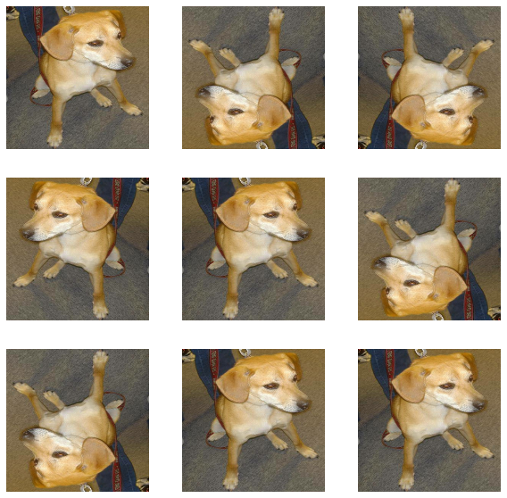
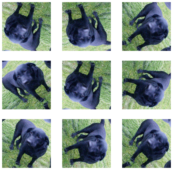
According to my PIC 16B HW 3 assignment page, ‘Data augmentation refers to the practice of including modified copies of the same image in the training set. ‘ We will be including both a tf.keras.layers.RandomFlip() layer and tf.keras.layers.RandomRotation(), so let’s explore these layers real quick! We will select a random image and apply different augmentations to it, as well as visualize these augmentations.
from keras.layers.preprocessing.image_preprocessing import RandomFlip

plt.figure(figsize=(10, 10))

for image, _ in train_dataset.take(1):
  for i in range(9):
    ax = plt.subplot(3, 3, i + 1)
    img_flip = tf.keras.layers.RandomFlip('horizontal_and_vertical')(tf.expand_dims(image[0], 0)) #randomly flips image
    plt.imshow(img_flip[0] / 255)
    plt.axis('off')
from keras.layers.preprocessing.image_preprocessing import RandomRotation

plt.figure(figsize=(10, 10))

for image, _ in train_dataset.take(1):
  for i in range(9):
    ax = plt.subplot(3, 3, i + 1)
    img_rot = tf.keras.layers.RandomRotation(0.5)(tf.expand_dims(image[0], 0)) #randomly rotates image
    plt.imshow(img_rot[0] / 255)
    plt.axis('off')
data_aug = tf.keras.Sequential([tf.keras.layers.RandomFlip("horizontal_and_vertical"),
                                tf.keras.Sequential(tf.keras.layers.RandomRotation(0.5))])

#apply randomflip and randomrotation to our data to use in model
aug_ds = train_dataset.map(lambda x, y: (data_aug(x, training=True), y))
After we’ve applied the augmentations to our training data, we will now build our new model and fit it to our augmented data.
model2 =  keras.models.Sequential([
    keras.layers.Reshape((160, 160, 3), input_shape = (160,160,3)),
    keras.layers.Conv2D(2, (3, 3), activation = 'relu'),
    keras.layers.MaxPooling2D((2,2)),
    keras.layers.Dense(units = 10, activation = 'selu'),
    keras.layers.Conv2D(2, (3, 3), activation = 'swish'),
    keras.layers.MaxPooling2D((2,2)),
    keras.layers.Flatten(),
    keras.layers.Dense(units = 30, activation = 'softmax'),
    keras.layers.Dropout(0.2)
    ])
model2.summary()
Model: "sequential_73"
_________________________________________________________________
 Layer (type)                Output Shape              Param #
=================================================================
 reshape_44 (Reshape)        (None, 160, 160, 3)       0

 conv2d_83 (Conv2D)          (None, 158, 158, 2)       56

 max_pooling2d_61 (MaxPoolin  (None, 79, 79, 2)        0
 g2D)

 dense_81 (Dense)            (None, 79, 79, 10)        30

 conv2d_84 (Conv2D)          (None, 77, 77, 2)         182

 max_pooling2d_62 (MaxPoolin  (None, 38, 38, 2)        0
 g2D)

 flatten_46 (Flatten)        (None, 2888)              0

 dense_82 (Dense)            (None, 30)                86670

 dropout_39 (Dropout)        (None, 30)                0

=================================================================
Total params: 86,938
Trainable params: 86,938
Non-trainable params: 0
_________________________________________________________________
model2.compile(optimizer='adam',
              loss=tf.keras.losses.SparseCategoricalCrossentropy(),
              metrics=['accuracy'])
history = model2.fit(aug_ds,
                     epochs=20,
                     validation_data=validation_dataset)
Epoch 1/20
63/63 [==============================] - 37s 571ms/step - loss: 4.0665 - accuracy: 0.4565 - val_loss: 1.3875 - val_accuracy: 0.4975
Epoch 2/20
63/63 [==============================] - 37s 576ms/step - loss: 3.1137 - accuracy: 0.4885 - val_loss: 0.9923 - val_accuracy: 0.5124
Epoch 3/20
63/63 [==============================] - 36s 572ms/step - loss: 3.2169 - accuracy: 0.4855 - val_loss: 0.8326 - val_accuracy: 0.5223
Epoch 4/20
63/63 [==============================] - 36s 572ms/step - loss: 2.8845 - accuracy: 0.5090 - val_loss: 0.8369 - val_accuracy: 0.5000
Epoch 5/20
63/63 [==============================] - 36s 572ms/step - loss: 3.1802 - accuracy: 0.4850 - val_loss: 0.7982 - val_accuracy: 0.4814
Epoch 6/20
63/63 [==============================] - 36s 571ms/step - loss: 3.0757 - accuracy: 0.4920 - val_loss: 0.7447 - val_accuracy: 0.4975
Epoch 7/20
63/63 [==============================] - 36s 566ms/step - loss: 3.0972 - accuracy: 0.4870 - val_loss: 0.7102 - val_accuracy: 0.5495
Epoch 8/20
63/63 [==============================] - 36s 565ms/step - loss: 3.1207 - accuracy: 0.4965 - val_loss: 0.7423 - val_accuracy: 0.5037
Epoch 9/20
63/63 [==============================] - 36s 571ms/step - loss: 3.3065 - accuracy: 0.4955 - val_loss: 0.7693 - val_accuracy: 0.5359
Epoch 10/20
63/63 [==============================] - 36s 569ms/step - loss: 2.9818 - accuracy: 0.5040 - val_loss: 0.7053 - val_accuracy: 0.5557
Epoch 11/20
63/63 [==============================] - 36s 569ms/step - loss: 2.9897 - accuracy: 0.5025 - val_loss: 0.7083 - val_accuracy: 0.5545
Epoch 12/20
63/63 [==============================] - 36s 566ms/step - loss: 2.9472 - accuracy: 0.5065 - val_loss: 0.7340 - val_accuracy: 0.5644
Epoch 13/20
63/63 [==============================] - 36s 567ms/step - loss: 2.7782 - accuracy: 0.5010 - val_loss: 0.6820 - val_accuracy: 0.5928
Epoch 14/20
63/63 [==============================] - 36s 568ms/step - loss: 2.9999 - accuracy: 0.5055 - val_loss: 0.8921 - val_accuracy: 0.4901
Epoch 15/20
63/63 [==============================] - 36s 566ms/step - loss: 3.1549 - accuracy: 0.5015 - val_loss: 0.7174 - val_accuracy: 0.5891
Epoch 16/20
63/63 [==============================] - 36s 564ms/step - loss: 3.0802 - accuracy: 0.5240 - val_loss: 0.7708 - val_accuracy: 0.5644
Epoch 17/20
63/63 [==============================] - 36s 571ms/step - loss: 3.0256 - accuracy: 0.5115 - val_loss: 0.7822 - val_accuracy: 0.5619
Epoch 18/20
63/63 [==============================] - 36s 571ms/step - loss: 3.1117 - accuracy: 0.4975 - val_loss: 0.6884 - val_accuracy: 0.5903
Epoch 19/20
63/63 [==============================] - 36s 571ms/step - loss: 3.0779 - accuracy: 0.5225 - val_loss: 0.7097 - val_accuracy: 0.5705
Epoch 20/20
63/63 [==============================] - 36s 569ms/step - loss: 3.1397 - accuracy: 0.5150 - val_loss: 0.7048 - val_accuracy: 0.5804
We achieved a final validation accuracy of 58.04%, with our highest validation accuracy being 59.28%, which means we reached our goal of obtaining at least a 55% accuracy rate!
The accuracy of my model stabilized between 53%-57%.
This model performed around the same as our first model.
The training and validation accuracy tended to stay around the same throughout, so, as a result, I would say the model is not overfitted.
§4. Data Preprocessing
i = tf.keras.Input(shape=(160, 160, 3))
x = tf.keras.applications.mobilenet_v2.preprocess_input(i)
preprocessor = tf.keras.Model(inputs = [i], outputs = [x])
For this model, we began by using our previous model’s layers, and then taking things out / adding layers to improve our accuracy rate! It’s suggested that we put the preprocessing layer first, then our augmentation layers, so that’s what we’ll do instead of applying the augmentation layers to our dataset!
When I tried building the mode with the previous model’s layers, I noticed I got low validation accuracies, so I decided to go back to the start and begin with a basic Conv2D layer with activation relu, and continue adding layers to improve the accuracy.
model3 = tf.keras.models.Sequential([
  preprocessor,
  keras.layers.RandomFlip("horizontal_and_vertical"),
  keras.layers.RandomRotation(0.2),
  keras.layers.Conv2D(32, (3, 3), activation='relu', input_shape=(160, 160, 3)),
  keras.layers.MaxPooling2D((2, 2)),
  keras.layers.Conv2D(32, (3, 3), activation='relu'),
  keras.layers.MaxPooling2D((2, 2)),
  keras.layers.Conv2D(64, (3,3), activation='relu'),
  keras.layers.MaxPooling2D((2, 2)),
  keras.layers.Dropout(0.2),
  keras.layers.Flatten(),
  keras.layers.Dense(64, activation='relu'),
  keras.layers.Dense(2),
])

model3.summary()
Model: "sequential_5"
_________________________________________________________________
 Layer (type)                Output Shape              Param #
=================================================================
 model (Functional)          (None, 160, 160, 3)       0

 random_flip_4 (RandomFlip)  (None, 160, 160, 3)       0

 random_rotation_4 (RandomRo  (None, 160, 160, 3)      0
 tation)

 conv2d_2 (Conv2D)           (None, 158, 158, 32)      896

 max_pooling2d_3 (MaxPooling  (None, 79, 79, 32)       0
 2D)

 conv2d_3 (Conv2D)           (None, 77, 77, 32)        9248

 max_pooling2d_4 (MaxPooling  (None, 38, 38, 32)       0
 2D)

 conv2d_4 (Conv2D)           (None, 36, 36, 64)        18496

 max_pooling2d_5 (MaxPooling  (None, 18, 18, 64)       0
 2D)

 dropout_1 (Dropout)         (None, 18, 18, 64)        0

 flatten_3 (Flatten)         (None, 20736)             0

 dense_8 (Dense)             (None, 64)                1327168

 dense_9 (Dense)             (None, 2)                 130

=================================================================
Total params: 1,355,938
Trainable params: 1,355,938
Non-trainable params: 0
_________________________________________________________________
model3.compile(optimizer='adam',
              loss=tf.keras.losses.SparseCategoricalCrossentropy(),
              metrics=['accuracy'])
history = model3.fit(train_data,
                     epochs=10,
                     validation_data=validation_dataset)
Epoch 1/20
63/63 [==============================] - 55s 824ms/step - loss: 3.1397 - accuracy: 0.5150 - val_loss: 0.7048 - val_accuracy: 0.5904
Epoch 2/20
63/63 [==============================] - 59s 930ms/step - loss: 0.6931 - accuracy: 0.5790 - val_loss: 0.6931 - val_accuracy: 0.6027
Epoch 3/20
63/63 [==============================] - 51s 808ms/step - loss: 0.6928 - accuracy: 0.5740 - val_loss: 0.6931 - val_accuracy: 0.6052
Epoch 4/20
63/63 [==============================] - 51s 804ms/step - loss: 0.6931 - accuracy: 0.5700 - val_loss: 0.6931 - val_accuracy: 0.6114
Epoch 5/20
63/63 [==============================] - 49s 783ms/step - loss: 0.6931 - accuracy: 0.5720 - val_loss: 0.6931 - val_accuracy: 0.6114
Epoch 6/20
63/63 [==============================] - 51s 815ms/step - loss: 0.6108 - accuracy: 0.6590 - val_loss: 0.6339 - val_accuracy: 0.6436
Epoch 7/20
63/63 [==============================] - 50s 794ms/step - loss: 0.6931 - accuracy: 0.5705 - val_loss: 0.6931 - val_accuracy: 0.6326
Epoch 8/20
63/63 [==============================] - 51s 815ms/step - loss: 0.6108 - accuracy: 0.6590 - val_loss: 0.6339 - val_accuracy: 0.6458
Epoch 9/20
63/63 [==============================] - 51s 805ms/step - loss: 0.5882 - accuracy: 0.6800 - val_loss: 0.6185 - val_accuracy: 0.6467
Epoch 10/20
63/63 [==============================] - 50s 790ms/step - loss: 0.5965 - accuracy: 0.6850 - val_loss: 0.6313 - val_accuracy: 0.6546
Epoch 11/20
63/63 [==============================] - 51s 811ms/step - loss: 0.5965 - accuracy: 0.6850 - val_loss: 0.6313 - val_accuracy: 0.6535
Epoch 12/20
63/63 [==============================] - 51s 815ms/step - loss: 0.6108 - accuracy: 0.6590 - val_loss: 0.6339 - val_accuracy: 0.6436
Epoch 13/20
63/63 [==============================] - 49s 783ms/step - loss: 0.5817 - accuracy: 0.6800 - val_loss: 0.6319 - val_accuracy: 0.6423
Epoch 14/20
63/63 [==============================] - 50s 785ms/step - loss: 0.6077 - accuracy: 0.6690 - val_loss: 0.6099 - val_accuracy: 0.6671
Epoch 15/20
63/63 [==============================] - 51s 790ms/step - loss: 0.5884 - accuracy: 0.6855 - val_loss: 0.5850 - val_accuracy: 0.6795
Epoch 16/20
63/63 [==============================] - 49s 789ms/step - loss: 0.5605 - accuracy: 0.7000 - val_loss: 0.6220 - val_accuracy: 0.6881
Epoch 17/20
63/63 [==============================] - 51s 818ms/step - loss: 0.5367 - accuracy: 0.7250 - val_loss: 0.5672 - val_accuracy: 0.7166
Epoch 18/20
63/63 [==============================] - 49s 782ms/step - loss: 0.5505 - accuracy: 0.7210 - val_loss: 0.5575 - val_accuracy: 0.7240
Epoch 19/20
63/63 [==============================] - 59s 930ms/step - loss: 0.5393 - accuracy: 0.7240 - val_loss: 0.5660 - val_accuracy: 0.7178
Epoch 20/20
63/63 [==============================] - 51s 808ms/step - loss: 0.5128 - accuracy: 0.7525 - val_loss: 0.5816 - val_accuracy: 0.7115
Our model ends with a validation accuracy of 0.7115, but the highest validation accuracy reached is about 0.7240. This means that our goal of achieving at least a 70% accuracy is reached!
Our validation accuracy for this model is definitely higher than that of model1. I would say this model is not overfitted; the training accuracies are within the same range of the validation accuracies; there is not a big difference between the two.
§5. Transfer Learning
For our final model, we will be using a base model (code below).
IMG_SHAPE = IMG_SIZE + (3,)
base_model = tf.keras.applications.MobileNetV2(input_shape=IMG_SHAPE,
                                               include_top=False,
                                               weights='imagenet')
base_model.trainable = False

i = tf.keras.Input(shape=IMG_SHAPE)
x = base_model(i, training = False)
base_model_layer = tf.keras.Model(inputs = [i], outputs = [x])
ALong with the base model, we will also be including our previous preprocessing layer, our data augmentation layers, and a Dense(2) layer to perform the classification.
model4 = tf.keras.models.Sequential([
      preprocessor,
      keras.layers.RandomFlip('horizontal_and_vertical'),
      keras.layers.RandomRotation(factor = (0.2)),
      base_model_layer,
      keras.layers.Flatten(),
      keras.layers.Dense(64, activation='relu'),
      keras.layers.Dense(2)
])

model4.summary()
Model: "sequential_6"
_________________________________________________________________
 Layer (type)                Output Shape              Param #
=================================================================
 model (Functional)          (None, 160, 160, 3)       0

 random_flip_5 (RandomFlip)  (None, 160, 160, 3)       0

 random_rotation_5 (RandomRo  (None, 160, 160, 3)      0
 tation)

 model_1 (Functional)        (None, 5, 5, 1280)        2257984

 flatten_4 (Flatten)         (None, 32000)             0

 dense_10 (Dense)            (None, 64)                2048064

 dense_11 (Dense)            (None, 2)                 130

=================================================================
Total params: 4,306,178
Trainable params: 2,048,194
Non-trainable params: 2,257,984
_________________________________________________________________
model4.compile(optimizer='adam',
              loss=tf.keras.losses.SparseCategoricalCrossentropy(),
              metrics=['accuracy'])
history = model4.fit(train_data,
                     epochs=20,
                     validation_data=validation_dataset)
Epoch 1/20
63/63 [==============================] - 55s 810ms/step - loss: 0.6814 - accuracy: 0.7865 - val_loss: 0.1432 - val_accuracy: 0.9493
Epoch 2/20
63/63 [==============================] - 49s 774ms/step - loss: 0.3834 - accuracy: 0.8825 - val_loss: 0.1317 - val_accuracy: 0.9542
Epoch 3/20
63/63 [==============================] - 50s 792ms/step - loss: 0.2694 - accuracy: 0.9165 - val_loss: 0.0806 - val_accuracy: 0.9691
Epoch 4/20
63/63 [==============================] - 49s 773ms/step - loss: 0.1969 - accuracy: 0.9185 - val_loss: 0.0698 - val_accuracy: 0.9765
Epoch 5/20
63/63 [==============================] - 51s 804ms/step - loss: 0.1516 - accuracy: 0.9340 - val_loss: 0.0619 - val_accuracy: 0.9777
Epoch 6/20
63/63 [==============================] - 56s 881ms/step - loss: 0.1481 - accuracy: 0.9475 - val_loss: 0.0760 - val_accuracy: 0.9752
Epoch 7/20
63/63 [==============================] - 53s 841ms/step - loss: 0.1403 - accuracy: 0.9475 - val_loss: 0.0993 - val_accuracy: 0.9629
Epoch 8/20
63/63 [==============================] - 55s 870ms/step - loss: 0.1419 - accuracy: 0.9465 - val_loss: 0.0757 - val_accuracy: 0.9752
Epoch 9/20
63/63 [==============================] - 51s 801ms/step - loss: 0.1333 - accuracy: 0.9485 - val_loss: 0.0699 - val_accuracy: 0.9765
Epoch 10/20
63/63 [==============================] - 49s 781ms/step - loss: 0.1230 - accuracy: 0.9495 - val_loss: 0.0853 - val_accuracy: 0.9678
Epoch 11/20
63/63 [==============================] - 48s 767ms/step - loss: 0.2012 - accuracy: 0.9325 - val_loss: 0.1139 - val_accuracy: 0.9691
Epoch 12/20
63/63 [==============================] - 48s 767ms/step - loss: 0.1135 - accuracy: 0.9535 - val_loss: 0.0810 - val_accuracy: 0.9703
Epoch 13/20
63/63 [==============================] - 48s 764ms/step - loss: 0.1090 - accuracy: 0.9580 - val_loss: 0.0723 - val_accuracy: 0.9740
Epoch 14/20
63/63 [==============================] - 49s 769ms/step - loss: 0.1095 - accuracy: 0.9510 - val_loss: 0.0697 - val_accuracy: 0.9802
Epoch 15/20
63/63 [==============================] - 49s 769ms/step - loss: 0.1194 - accuracy: 0.9505 - val_loss: 0.0993 - val_accuracy: 0.9604
Epoch 16/20
63/63 [==============================] - 49s 783ms/step - loss: 0.0979 - accuracy: 0.9590 - val_loss: 0.1068 - val_accuracy: 0.9567
Epoch 17/20
63/63 [==============================] - 49s 783ms/step - loss: 0.0896 - accuracy: 0.9665 - val_loss: 0.0927 - val_accuracy: 0.9691
Epoch 18/20
63/63 [==============================] - 49s 772ms/step - loss: 0.0838 - accuracy: 0.9655 - val_loss: 0.0939 - val_accuracy: 0.9715
Epoch 19/20
63/63 [==============================] - 48s 768ms/step - loss: 0.2199 - accuracy: 0.9265 - val_loss: 0.0859 - val_accuracy: 0.9703
Epoch 20/20
63/63 [==============================] - 48s 767ms/step - loss: 0.2122 - accuracy: 0.9250 - val_loss: 0.1023 - val_accuracy: 0.9666
We ended with a validation accuracy of about 96.7%, with our highest validation accuracy being about 98.02%! This means we achieved our goal of getting at least a 95% accuracy!
This model is the best performing one so far; it performed better than our past three models. There doesn’t appear to be any overfitting; the training accuracy and validation accuracy scores are very similar / within the same range of values.
§6. Score on Test Data
Since the model with the best validation accuracy is model 4, we will evaluate it on our test dataset to see how it performs.
model4.evaluate(test_dataset)
6/6 [==============================] - 4s 499ms/step - loss: 0.0959 - accuracy: 0.9774
Model 4 performed very well, getting an accuracy of about 97%!
Thank you so much for reading!