Classifying Fake News with Tensorflow
Introduction
Hello Everyone!
Today we will be learning how to classify fake news with Tensorflow! Let’s begin by importing the necessary packages and data.
Importing necessary packages and data
import numpy as np
import pandas as pd
import tensorflow as tf
import re
import string
import nltk
nltk.download('stopwords')
from nltk.corpus import stopwords

from tensorflow.keras import layers
from tensorflow.keras import losses

from tensorflow.keras.layers.experimental.preprocessing import TextVectorization
from tensorflow.keras.layers.experimental.preprocessing import StringLookup

from sklearn.model_selection import train_test_split
[nltk_data] Downloading package stopwords to /root/nltk_data...
[nltk_data]   Package stopwords is already up-to-date!
train_url = "https://github.com/PhilChodrow/PIC16b/blob/master/datasets/fake_news_train.csv?raw=true"

train_data = pd.read_csv(train_url)
train_data
The data we are importing contains article titles, text, and a column telling us if they are fake news or not.
| Unnamed: 0 | title | text | fake | |
|---|---|---|---|---|
| 0 | 17366 | Merkel: Strong result for Austria's FPO 'big c... | German Chancellor Angela Merkel said on Monday... | 0 |
| 1 | 5634 | Trump says Pence will lead voter fraud panel | WEST PALM BEACH, Fla.President Donald Trump sa... | 0 |
| 2 | 17487 | JUST IN: SUSPECTED LEAKER and “Close Confidant... | On December 5, 2017, Circa s Sara Carter warne... | 1 |
| 3 | 12217 | Thyssenkrupp has offered help to Argentina ove... | Germany s Thyssenkrupp, has offered assistance... | 0 |
| 4 | 5535 | Trump say appeals court decision on travel ban... | President Donald Trump on Thursday called the ... | 0 |
| ... | ... | ... | ... | ... |
| 22444 | 10709 | ALARMING: NSA Refuses to Release Clinton-Lynch... | If Clinton and Lynch just talked about grandki... | 1 |
| 22445 | 8731 | Can Pence's vow not to sling mud survive a Tru... | () - In 1990, during a close and bitter congre... | 0 |
| 22446 | 4733 | Watch Trump Campaign Try To Spin Their Way Ou... | A new ad by the Hillary Clinton SuperPac Prior... | 1 |
| 22447 | 3993 | Trump celebrates first 100 days as president, ... | HARRISBURG, Pa.U.S. President Donald Trump hit... | 0 |
| 22448 | 12896 | TRUMP SUPPORTERS REACT TO DEBATE: “Clinton New... | MELBOURNE, FL is a town with a population of 7... | 1 |
22449 rows × 4 columns
Next, we will be making a function to turn our data into a tensor object! This will allow us to create our models.
Make function to make data tensor object
Our function will first remove stopwords from our titles and text, and then we will turn it into a tensor object. Title and text will be our input, and fake will be our output.
def make_dataset(df):
  # Remove stopwords from the article text and title.
  # A stopword is a word that is usually considered to be uninformative, such as “the,” “and,” or “but.”
  # Construct and return a tf.data.Dataset with two inputs and one output. The input should be of the form (title, text),
  # and the output should consist only of the fake column. You may find it helpful to consult lecture notes or this tutorial for
  # reference on how to construct and use Datasets with multiple inputs

  #stop words
  stop = stopwords.words('english')

  #remove stop words from article title
  df["title"] = df['title'].apply(lambda x: ' '.join([word for word in x.split() if word not in (stop)]))
  #remove stop words from article text
  df["text"] = df['text'].apply(lambda x: ' '.join([word for word in x.split() if word not in (stop)]))

  data = tf.data.Dataset.from_tensor_slices(
   ( # dictionary for input data/features
    #our two inputs: title and text
    { "title": df[["title"]],
     "text": df["text"]
    },
    # dictionary for output data/labels
    # one output: fake
    { "fake": df[["fake"]]

    }
   )
  )

  return data.batch(100)
#batch our data to make training faster; train on chunks of data rather than individual rows
data = make_dataset(train_data)
#check size of dataset
len(data)
225
Now, we will be splitting our data into a training and validation set. Our validation set will be 20% of the data.
Split data into training and validation sets
#shuffle dataset
import random
random.seed(10)
data = data.shuffle(buffer_size = len(data))

#20% validation
val_size  = int(0.2*len(data))

val = data.take(val_size)
train = data.skip(val_size).take(len(data) - val_size)

#check size of training and validation sets
print(len(train), len(val))
180 45
Base rate - Labels Iterator, fake text, count of labels, on training data
Now, let’s look at our base rate by looking at the “fake” labels in our training data.
# Base rate
## similar to previous hw; can get true and fake from training data, labels iterator on fake column

labels_iterator= train.unbatch().map(lambda input, output: output).as_numpy_iterator()

train_data2 = train_data.sample(n=1800)

len(train_data2[train_data2["fake"] == 1]) / 1800
0.5355555555555556
The base rate appears to be about 53.6%, which indicates that a little more than half of the artiles in the training data is fake while the other half is true.
Model Creation
Next we will create our models, but before we do so, we must perform standardization and text vectorization.
# Text vectorization

#preparing a text vectorization layer for tf model
size_vocabulary = 2000

def standardization(input_data):
    lowercase = tf.strings.lower(input_data)
    no_punctuation = tf.strings.regex_replace(lowercase,
                                  '[%s]' % re.escape(string.punctuation),'')
    return no_punctuation

## Title Vectorization
title_vectorize_layer = TextVectorization(
    standardize=standardization,
    max_tokens=size_vocabulary, # only consider this many words
    output_mode='int',
    output_sequence_length=500)

title_vectorize_layer.adapt(train.map(lambda x, y: x["title"]))

## Text Vectorization

text_vectorize_layer = TextVectorization(
    standardize=standardization,
    max_tokens=size_vocabulary,
    output_mode='int',
    output_sequence_length=500)

text_vectorize_layer.adapt(train.map(lambda x, y: x["text"]))
We will be creating 3 models: one with the title only, one with the text only, and one with both the text and title. The purpose of this is to see which method will classify fake news the best.
Model 1: Title only
For our first model, we will focus on just using the title. We must first create an input.
title_input = tf.keras.Input(
    shape=(1,),
    name = "title", # same name as the dictionary key in the dataset
    dtype = "string"
)
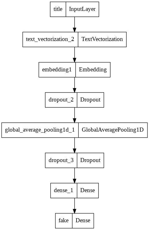
Next, we will add our layers. Since our titles are categorical and not numerical, we will add GlobalAveragePooling. For this, we will include an embedding and begin with 0.2 for our dropout. I decided to begin with these parameters based on the lecture notes.
# layers for processing the title
title_features = title_vectorize_layer(title_input)

# Add embedding layer, dropout
title_features = layers.Embedding(size_vocabulary, output_dim = 3, name="embedding1")(title_features)
title_features = layers.Dropout(0.2)(title_features)
title_features = layers.GlobalAveragePooling1D()(title_features)
title_features = layers.Dropout(0.2)(title_features)
title_features = layers.Dense(2, activation='relu')(title_features)

output = layers.Dense(2, name="fake")(title_features)
Now, we create our model and check its summary.
model1 = tf.keras.Model(
    inputs = title_input,
    outputs = output
)
from tensorflow.keras import utils

model1.summary()
utils.plot_model(model1)
Model: "model_1"
_________________________________________________________________
 Layer (type)                Output Shape              Param #
=================================================================
 title (InputLayer)          [(None, 1)]               0

 text_vectorization_2 (TextV  (None, 500)              0
 ectorization)

 embedding1 (Embedding)      (None, 500, 3)            6000

 dropout_2 (Dropout)         (None, 500, 3)            0

 global_average_pooling1d_1   (None, 3)                0
 (GlobalAveragePooling1D)

 dropout_3 (Dropout)         (None, 3)                 0

 dense_1 (Dense)             (None, 2)                 8

 fake (Dense)                (None, 2)                 6

=================================================================
Total params: 6,014
Trainable params: 6,014
Non-trainable params: 0
_________________________________________________________________
model1.compile(optimizer="adam",
              loss = losses.SparseCategoricalCrossentropy(from_logits=True),
              metrics=["accuracy"])
Now, let’s fit our data.
history = model1.fit(train, validation_data=val, epochs=20)
Epoch 1/20


/usr/local/lib/python3.7/dist-packages/keras/engine/functional.py:559: UserWarning: Input dict contained keys ['text'] which did not match any model input. They will be ignored by the model.
  inputs = self._flatten_to_reference_inputs(inputs)


180/180 [==============================] - 3s 11ms/step - loss: 0.6922 - accuracy: 0.5199 - val_loss: 0.6909 - val_accuracy: 0.5244
Epoch 2/20
180/180 [==============================] - 2s 9ms/step - loss: 0.6889 - accuracy: 0.5577 - val_loss: 0.6845 - val_accuracy: 0.5988
Epoch 3/20
180/180 [==============================] - 2s 9ms/step - loss: 0.6764 - accuracy: 0.6732 - val_loss: 0.6650 - val_accuracy: 0.8622
Epoch 4/20
180/180 [==============================] - 2s 9ms/step - loss: 0.6485 - accuracy: 0.8005 - val_loss: 0.6267 - val_accuracy: 0.9313
Epoch 5/20
180/180 [==============================] - 2s 10ms/step - loss: 0.6015 - accuracy: 0.8615 - val_loss: 0.5699 - val_accuracy: 0.9285
Epoch 6/20
180/180 [==============================] - 2s 9ms/step - loss: 0.5442 - accuracy: 0.8794 - val_loss: 0.5050 - val_accuracy: 0.9322
Epoch 7/20
180/180 [==============================] - 2s 10ms/step - loss: 0.4829 - accuracy: 0.8984 - val_loss: 0.4426 - val_accuracy: 0.9338
Epoch 8/20
180/180 [==============================] - 2s 9ms/step - loss: 0.4248 - accuracy: 0.9200 - val_loss: 0.3848 - val_accuracy: 0.9338
Epoch 9/20
180/180 [==============================] - 2s 10ms/step - loss: 0.3756 - accuracy: 0.9275 - val_loss: 0.3347 - val_accuracy: 0.9520
Epoch 10/20
180/180 [==============================] - 2s 13ms/step - loss: 0.3306 - accuracy: 0.9383 - val_loss: 0.2911 - val_accuracy: 0.9531
Epoch 11/20
180/180 [==============================] - 2s 10ms/step - loss: 0.2931 - accuracy: 0.9438 - val_loss: 0.2575 - val_accuracy: 0.9642
Epoch 12/20
180/180 [==============================] - 2s 10ms/step - loss: 0.2606 - accuracy: 0.9494 - val_loss: 0.2229 - val_accuracy: 0.9651
Epoch 13/20
180/180 [==============================] - 2s 10ms/step - loss: 0.2355 - accuracy: 0.9514 - val_loss: 0.1958 - val_accuracy: 0.9671
Epoch 14/20
180/180 [==============================] - 2s 9ms/step - loss: 0.2149 - accuracy: 0.9535 - val_loss: 0.1829 - val_accuracy: 0.9667
Epoch 15/20
180/180 [==============================] - 2s 10ms/step - loss: 0.1938 - accuracy: 0.9570 - val_loss: 0.1662 - val_accuracy: 0.9700
Epoch 16/20
180/180 [==============================] - 2s 10ms/step - loss: 0.1809 - accuracy: 0.9582 - val_loss: 0.1478 - val_accuracy: 0.9718
Epoch 17/20
180/180 [==============================] - 2s 10ms/step - loss: 0.1665 - accuracy: 0.9608 - val_loss: 0.1375 - val_accuracy: 0.9684
Epoch 18/20
180/180 [==============================] - 2s 10ms/step - loss: 0.1552 - accuracy: 0.9621 - val_loss: 0.1265 - val_accuracy: 0.9693
Epoch 19/20
180/180 [==============================] - 2s 11ms/step - loss: 0.1441 - accuracy: 0.9630 - val_loss: 0.1164 - val_accuracy: 0.9747
Epoch 20/20
180/180 [==============================] - 2s 10ms/step - loss: 0.1364 - accuracy: 0.9666 - val_loss: 0.1104 - val_accuracy: 0.9747
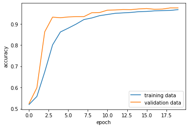
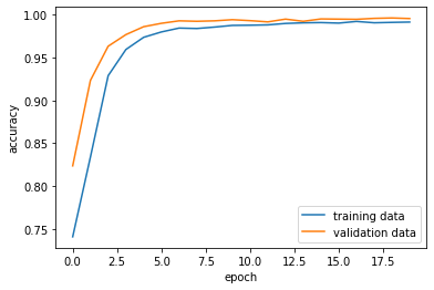
As we can see, we have a pretty good validation accuracy (around 97%) and the models don’t appear to be overfitted! Let’s visualize this process then move onto our next model.
from matplotlib import pyplot as plt
plt.plot(history.history["accuracy"], label="training data")
plt.plot(history.history["val_accuracy"], label="validation data")
plt.gca().set(xlabel = "epoch", ylabel = "accuracy")
plt.legend()
Model 2: Text Only
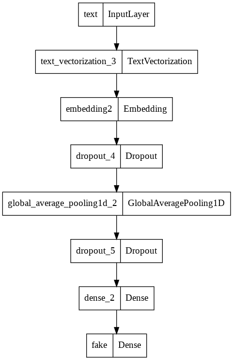
Our next model is using just text. We repeat the same process as above, but with the text instead of titles.
text_input = tf.keras.Input(
    shape=(1,),
    name = "text",
    dtype = "string"
)
For our layers, I initially tried the same parameters as the title model, but decided to try 0.3 and 0.4 for the dropout because the model seemed to be a bit overfitted. 0.4 had the best accuracy rates, so I went with that one! After this, let’s fit our model and visualize it.
# layers for processing the title
text_features = text_vectorize_layer(text_input)

# Add embedding layer, dropout
text_features = layers.Embedding(size_vocabulary, output_dim = 3, name="embedding2")(text_features)
text_features = layers.Dropout(0.4)(text_features)
text_features = layers.GlobalAveragePooling1D()(text_features)
text_features = layers.Dropout(0.4)(text_features)
text_features = layers.Dense(2, activation='relu')(text_features)

output = layers.Dense(2, name="fake")(text_features)
model2 = tf.keras.Model(
    inputs = text_input,
    outputs = output
)
from tensorflow.keras import utils

model2.summary()
utils.plot_model(model2)
Model: "model_2"
_________________________________________________________________
 Layer (type)                Output Shape              Param #
=================================================================
 text (InputLayer)           [(None, 1)]               0

 text_vectorization_3 (TextV  (None, 500)              0
 ectorization)

 embedding2 (Embedding)      (None, 500, 3)            6000

 dropout_4 (Dropout)         (None, 500, 3)            0

 global_average_pooling1d_2   (None, 3)                0
 (GlobalAveragePooling1D)

 dropout_5 (Dropout)         (None, 3)                 0

 dense_2 (Dense)             (None, 2)                 8

 fake (Dense)                (None, 2)                 6

=================================================================
Total params: 6,014
Trainable params: 6,014
Non-trainable params: 0
_________________________________________________________________
model2.compile(optimizer="adam",
              loss = losses.SparseCategoricalCrossentropy(from_logits=True),
              metrics=["accuracy"])
history = model2.fit(train, validation_data=val, epochs=20)
Epoch 1/20


/usr/local/lib/python3.7/dist-packages/keras/engine/functional.py:559: UserWarning: Input dict contained keys ['title'] which did not match any model input. They will be ignored by the model.
  inputs = self._flatten_to_reference_inputs(inputs)


180/180 [==============================] - 4s 19ms/step - loss: 0.6907 - accuracy: 0.5299 - val_loss: 0.6852 - val_accuracy: 0.5364
Epoch 2/20
180/180 [==============================] - 3s 18ms/step - loss: 0.6636 - accuracy: 0.7319 - val_loss: 0.6298 - val_accuracy: 0.8787
Epoch 3/20
180/180 [==============================] - 3s 18ms/step - loss: 0.5893 - accuracy: 0.8307 - val_loss: 0.5279 - val_accuracy: 0.9204
Epoch 4/20
180/180 [==============================] - 3s 17ms/step - loss: 0.4990 - accuracy: 0.8798 - val_loss: 0.4294 - val_accuracy: 0.9272
Epoch 5/20
180/180 [==============================] - 3s 17ms/step - loss: 0.4213 - accuracy: 0.9020 - val_loss: 0.3582 - val_accuracy: 0.9516
Epoch 6/20
180/180 [==============================] - 3s 17ms/step - loss: 0.3631 - accuracy: 0.9121 - val_loss: 0.2960 - val_accuracy: 0.9602
Epoch 7/20
180/180 [==============================] - 4s 22ms/step - loss: 0.3200 - accuracy: 0.9188 - val_loss: 0.2558 - val_accuracy: 0.9567
Epoch 8/20
180/180 [==============================] - 3s 18ms/step - loss: 0.2850 - accuracy: 0.9242 - val_loss: 0.2293 - val_accuracy: 0.9595
Epoch 9/20
180/180 [==============================] - 4s 19ms/step - loss: 0.2611 - accuracy: 0.9284 - val_loss: 0.2031 - val_accuracy: 0.9676
Epoch 10/20
180/180 [==============================] - 3s 19ms/step - loss: 0.2408 - accuracy: 0.9313 - val_loss: 0.1800 - val_accuracy: 0.9691
Epoch 11/20
180/180 [==============================] - 3s 18ms/step - loss: 0.2269 - accuracy: 0.9288 - val_loss: 0.1676 - val_accuracy: 0.9691
Epoch 12/20
180/180 [==============================] - 3s 17ms/step - loss: 0.2123 - accuracy: 0.9371 - val_loss: 0.1555 - val_accuracy: 0.9684
Epoch 13/20
180/180 [==============================] - 3s 19ms/step - loss: 0.1982 - accuracy: 0.9368 - val_loss: 0.1382 - val_accuracy: 0.9731
Epoch 14/20
180/180 [==============================] - 3s 18ms/step - loss: 0.1908 - accuracy: 0.9388 - val_loss: 0.1335 - val_accuracy: 0.9717
Epoch 15/20
180/180 [==============================] - 3s 17ms/step - loss: 0.1822 - accuracy: 0.9383 - val_loss: 0.1325 - val_accuracy: 0.9720
Epoch 16/20
180/180 [==============================] - 3s 18ms/step - loss: 0.1768 - accuracy: 0.9361 - val_loss: 0.1191 - val_accuracy: 0.9753
Epoch 17/20
180/180 [==============================] - 3s 18ms/step - loss: 0.1724 - accuracy: 0.9398 - val_loss: 0.1058 - val_accuracy: 0.9776
Epoch 18/20
180/180 [==============================] - 3s 17ms/step - loss: 0.1653 - accuracy: 0.9404 - val_loss: 0.1061 - val_accuracy: 0.9773
Epoch 19/20
180/180 [==============================] - 3s 18ms/step - loss: 0.1639 - accuracy: 0.9401 - val_loss: 0.0997 - val_accuracy: 0.9782
Epoch 20/20
180/180 [==============================] - 3s 17ms/step - loss: 0.1585 - accuracy: 0.9399 - val_loss: 0.0978 - val_accuracy: 0.9802
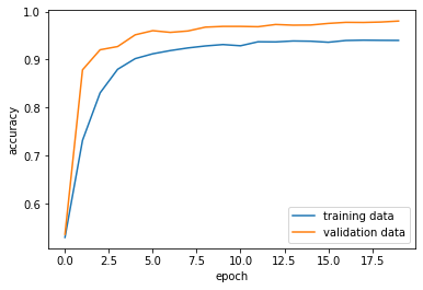
As we can see, the validation accuracy is pretty high, sitting at around 98%! This looks promising, but let’s try our final model.
plt.plot(history.history["accuracy"], label="training data")
plt.plot(history.history["val_accuracy"], label="validation data")
plt.gca().set(xlabel = "epoch", ylabel = "accuracy")
plt.legend()
Model 3: Title and Text
Now, we create a model that uses both the title and text. We begin by concatenating our title and text feattures.
main = layers.concatenate([title_features, text_features], axis = 1)
Next, we will create layers for this concatenation and use it for our output.
main = layers.Dense(4, activation='relu')(main)
output = layers.Dense(4, name="fake")(main)
model3 = tf.keras.Model(
    inputs = [title_input, text_input],
    outputs = output
)
model3.compile(optimizer="adam",
              loss = losses.SparseCategoricalCrossentropy(from_logits=True),
              metrics=["accuracy"])
history = model3.fit(train,
                    validation_data=val,
                    epochs = 20)
Epoch 1/20
180/180 [==============================] - 8s 40ms/step - loss: 1.0807 - accuracy: 0.7412 - val_loss: 0.8972 - val_accuracy: 0.8238
Epoch 2/20
180/180 [==============================] - 4s 22ms/step - loss: 0.8153 - accuracy: 0.8341 - val_loss: 0.6897 - val_accuracy: 0.9233
Epoch 3/20
180/180 [==============================] - 4s 22ms/step - loss: 0.6401 - accuracy: 0.9288 - val_loss: 0.5430 - val_accuracy: 0.9631
Epoch 4/20
180/180 [==============================] - 4s 22ms/step - loss: 0.5208 - accuracy: 0.9593 - val_loss: 0.4383 - val_accuracy: 0.9766
Epoch 5/20
180/180 [==============================] - 4s 21ms/step - loss: 0.4267 - accuracy: 0.9735 - val_loss: 0.3624 - val_accuracy: 0.9858
Epoch 6/20
180/180 [==============================] - 4s 21ms/step - loss: 0.3540 - accuracy: 0.9797 - val_loss: 0.2913 - val_accuracy: 0.9898
Epoch 7/20
180/180 [==============================] - 4s 21ms/step - loss: 0.2939 - accuracy: 0.9842 - val_loss: 0.2426 - val_accuracy: 0.9927
Epoch 8/20
180/180 [==============================] - 4s 21ms/step - loss: 0.2490 - accuracy: 0.9837 - val_loss: 0.2031 - val_accuracy: 0.9921
Epoch 9/20
180/180 [==============================] - 4s 22ms/step - loss: 0.2139 - accuracy: 0.9854 - val_loss: 0.1734 - val_accuracy: 0.9927
Epoch 10/20
180/180 [==============================] - 4s 21ms/step - loss: 0.1824 - accuracy: 0.9874 - val_loss: 0.1494 - val_accuracy: 0.9940
Epoch 11/20
180/180 [==============================] - 4s 22ms/step - loss: 0.1607 - accuracy: 0.9876 - val_loss: 0.1281 - val_accuracy: 0.9929
Epoch 12/20
180/180 [==============================] - 4s 21ms/step - loss: 0.1408 - accuracy: 0.9880 - val_loss: 0.1161 - val_accuracy: 0.9915
Epoch 13/20
180/180 [==============================] - 4s 22ms/step - loss: 0.1216 - accuracy: 0.9896 - val_loss: 0.0978 - val_accuracy: 0.9947
Epoch 14/20
180/180 [==============================] - 4s 21ms/step - loss: 0.1098 - accuracy: 0.9904 - val_loss: 0.0926 - val_accuracy: 0.9921
Epoch 15/20
180/180 [==============================] - 4s 21ms/step - loss: 0.0972 - accuracy: 0.9906 - val_loss: 0.0795 - val_accuracy: 0.9949
Epoch 16/20
180/180 [==============================] - 4s 22ms/step - loss: 0.0895 - accuracy: 0.9900 - val_loss: 0.0719 - val_accuracy: 0.9947
Epoch 17/20
180/180 [==============================] - 4s 22ms/step - loss: 0.0786 - accuracy: 0.9920 - val_loss: 0.0666 - val_accuracy: 0.9944
Epoch 18/20
180/180 [==============================] - 4s 22ms/step - loss: 0.0724 - accuracy: 0.9904 - val_loss: 0.0542 - val_accuracy: 0.9956
Epoch 19/20
180/180 [==============================] - 4s 21ms/step - loss: 0.0676 - accuracy: 0.9909 - val_loss: 0.0494 - val_accuracy: 0.9960
Epoch 20/20
180/180 [==============================] - 7s 37ms/step - loss: 0.0627 - accuracy: 0.9913 - val_loss: 0.0469 - val_accuracy: 0.9953
As we can see, this model performed the best, sitting at 99.5%!
from matplotlib import pyplot as plt
plt.plot(history.history["accuracy"], label="training data")
plt.plot(history.history["val_accuracy"], label="validation data")
plt.gca().set(xlabel = "epoch", ylabel = "accuracy")
plt.legend()
Looking at all of our models, it appears that the model using both text and title scored the highest and is our best model! This makes sense, as using both the text and title gives our model more information to learn from and thus may be more helpful. Let’s evaluate our model using test data and see how it performs!
Model Evaluation on Test Data
Let’s read in our test data.
test_url = "https://github.com/PhilChodrow/PIC16b/blob/master/datasets/fake_news_test.csv?raw=true"

test_data = pd.read_csv(test_url)
test_data

test = make_dataset(test_data)
Now, we will evaluate our best model on the testing data:
test_evaluate = model3.evaluate(test)
225/225 [==============================] - 3s 12ms/step - loss: 0.0541 - accuracy: 0.9930
We get an accuracy of about 99.3%. This tells us that the model performed very well; if we used the model as a fake news predictor, we would be right about 99.3% of the time.
Now, let’s create an embedding visualization.
Embedding Visualization
weights = model2.get_layer('embedding2').get_weights()[0] # get the weights from the embedding layer
vocab = text_vectorize_layer.get_vocabulary()                # get the vocabulary from our data prep for later

from sklearn.decomposition import PCA
pca = PCA(n_components=2)
weights = pca.fit_transform(weights)

embedding_df = pd.DataFrame({
    'word' : vocab,
    'x0'   : weights[:,0],
    'x1'   : weights[:,1]
})
import plotly.express as px
fig = px.scatter(embedding_df,
                 x = "x0",
                 y = "x1",
                 size = [2]*len(embedding_df),
                # size_max = 2,
                 hover_name = "word")

fig.show()
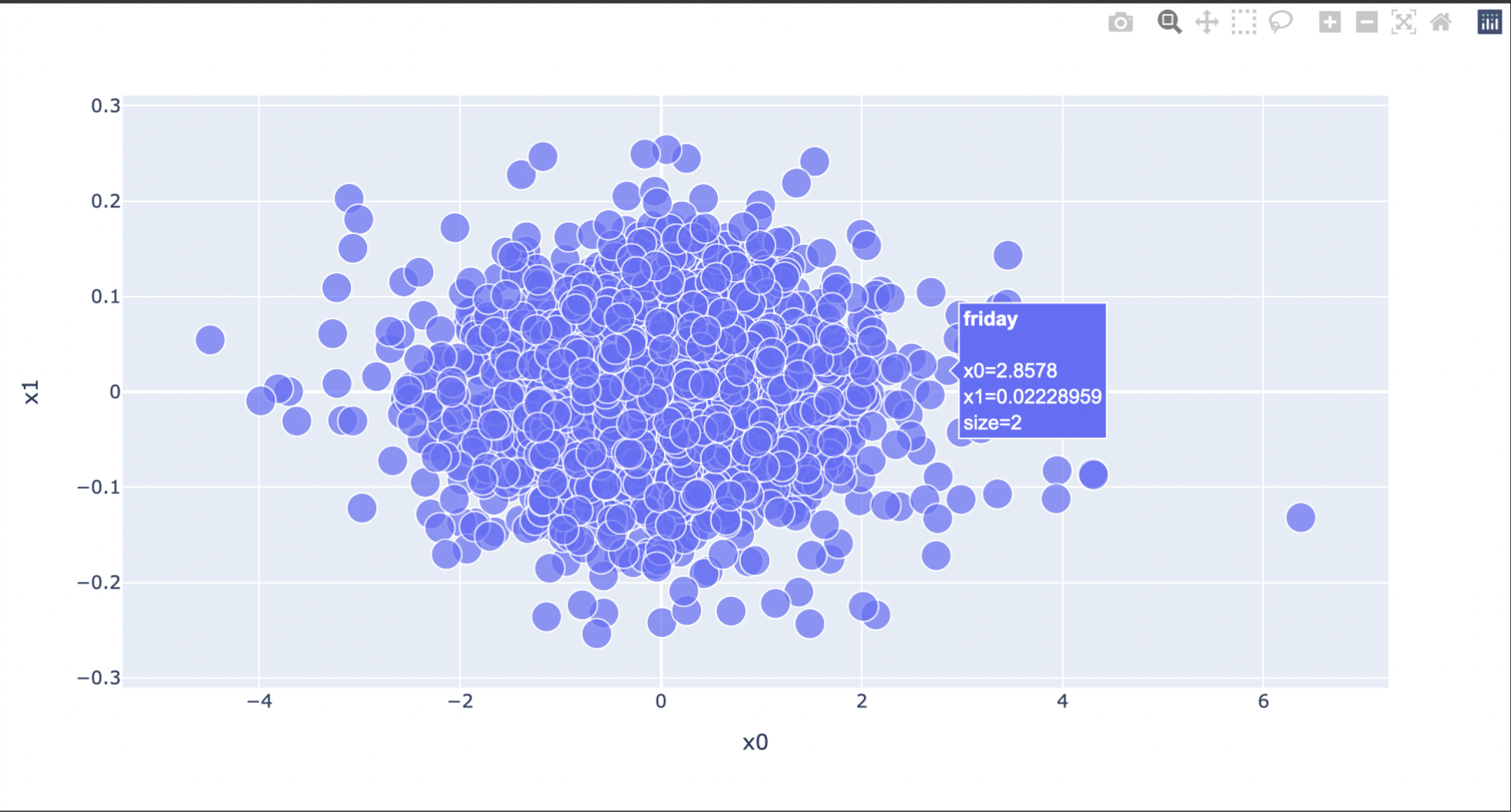
Five words that I found interpretable and interesting in this visualization are “apparently,” “fox,” “reportedly,” “radical,” and “21wire,” all of which reside towards the left side of the visualization. “fox” and “21wire” most likely refers to Fox News and 21st Century Wire, which are both news sources that have been criticized for spreading propoganda and false or exhaggerated information. “apparently” and “reportedly” also make sense to me because these are words that are often used by writers when they can’t be sure about the information; these words allow them to detach themselves from involvement. “radical” also makes sense as a fake news word because a lot of fake news articles tend to attack “radical leftists.”
That’s it for today! Thank you so much for reading!