Predicting Penguin Species Using Machine Learning Models
Introduction
Hello everyone!
Today we’ll be predicitng penguin species using machine learning models. We’ll be using the Palmer’s Penguins dataset for this task.
Data Import and Cleaning
We will begin by importing our data and splitting our data into training and testing sets for both X (predictor variables) and y (target variable), as well as importing all the relevant packages needed. Once we’ve split the data, we will inspect our variables with missing values and remove rows with the values.
#import relevant packages for project
import pandas as pd
from matplotlib import pyplot as plt
import numpy as np
from sklearn.model_selection import train_test_split
from sklearn import preprocessing
import seaborn as sns

#import our data
penguins=pd.read_csv("palmer_penguins.csv")

#checks first five rows of our data
penguins.head()
| studyName | Sample Number | Species | Region | Island | Stage | Individual ID | Clutch Completion | Date Egg | Culmen Length (mm) | Culmen Depth (mm) | Flipper Length (mm) | Body Mass (g) | Sex | Delta 15 N (o/oo) | Delta 13 C (o/oo) | Comments | |
|---|---|---|---|---|---|---|---|---|---|---|---|---|---|---|---|---|---|
| 0 | PAL0708 | 1 | Adelie Penguin (Pygoscelis adeliae) | Anvers | Torgersen | Adult, 1 Egg Stage | N1A1 | Yes | 11/11/07 | 39.1 | 18.7 | 181.0 | 3750.0 | MALE | NaN | NaN | Not enough blood for isotopes. |
| 1 | PAL0708 | 2 | Adelie Penguin (Pygoscelis adeliae) | Anvers | Torgersen | Adult, 1 Egg Stage | N1A2 | Yes | 11/11/07 | 39.5 | 17.4 | 186.0 | 3800.0 | FEMALE | 8.94956 | -24.69454 | NaN |
| 2 | PAL0708 | 3 | Adelie Penguin (Pygoscelis adeliae) | Anvers | Torgersen | Adult, 1 Egg Stage | N2A1 | Yes | 11/16/07 | 40.3 | 18.0 | 195.0 | 3250.0 | FEMALE | 8.36821 | -25.33302 | NaN |
| 3 | PAL0708 | 4 | Adelie Penguin (Pygoscelis adeliae) | Anvers | Torgersen | Adult, 1 Egg Stage | N2A2 | Yes | 11/16/07 | NaN | NaN | NaN | NaN | NaN | NaN | NaN | Adult not sampled. |
| 4 | PAL0708 | 5 | Adelie Penguin (Pygoscelis adeliae) | Anvers | Torgersen | Adult, 1 Egg Stage | N3A1 | Yes | 11/16/07 | 36.7 | 19.3 | 193.0 | 3450.0 | FEMALE | 8.76651 | -25.32426 | NaN |
</div>
#check dimensions of our data
penguins.shape
(344, 17)
#removes single row where Sex is "."
penguins = penguins[-(penguins["Sex"] == ".")]
penguins.shape
(343, 17)
We will first inspect which variables have the most missing values and get rid of them so we aren’t left with an incredibly small dataset when we drop rows with missing values.
plt.figure(figsize=(10,6))
sns.displot(
    data=penguins.isna().melt(value_name="missing"),
    y="variable",
    hue="missing",
    multiple="fill"
)
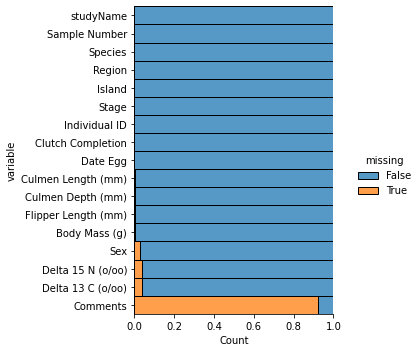
As we can see, “Comments” has a large amount of missing values; it accounts for almost all the data within the column! Thus, we will initially remove the “Comments” column from the data so that when we remove missing values, we aren’t left with only a few rows. Delta 15N, Delta 13C, and Sex also appear to have a good amount of missing values as well, but the missing values only accounts for about 4% of the data in each column, so we can just get rid of them rather than impute them.
#alter dataset so that we no longer have the Comments column
penguins=penguins.drop("Comments", axis=1)
#check to see that the Comments column has been removed
penguins.shape
(343, 16)
Next, we will be splitting the data into testing (20%) and training (80%) sets before we further clean the data.
np.random.seed(1128)
#split into testing and training data
train,test=train_test_split(penguins,test_size=.20)

def prep_data(data):
    '''Takes inputted data and splits it into target and predictor variables

    @param data: datafram
    @return: target and predictor variables
    '''

    #make copy of data
    df = data.copy()

    #predictor variables
    X = df.drop(["Species"], axis = 1)
    #target variable
    y = df["Species"]

    return(X, y)
Let’s first get rid of our missing values in each set then split the data.
#drop missing values from training data
train = train.dropna()
#drop missing values from testing data
test= test.dropna()

#split testing and training into predictor and target variables
X_train, y_train = prep_data(train)
X_test,  y_test  = prep_data(test)

#check dimensions of split data
X_train.shape, X_test.shape, y_train.shape, y_test.shape
((258, 15), (66, 15), (258,), (66,))
Exploratory Data Analysis
Next, we will be performing exploratory data analysis on the predictor variables in our training set to help us narrow down significant variables.
#observe the training data
X_train.head()
| studyName | Sample Number | Region | Island | Stage | Individual ID | Clutch Completion | Date Egg | Culmen Length (mm) | Culmen Depth (mm) | Flipper Length (mm) | Body Mass (g) | Sex | Delta 15 N (o/oo) | Delta 13 C (o/oo) | |
|---|---|---|---|---|---|---|---|---|---|---|---|---|---|---|---|
| 228 | PAL0708 | 9 | Anvers | Biscoe | Adult, 1 Egg Stage | N35A1 | Yes | 11/27/07 | 43.3 | 13.4 | 209.0 | 4400.0 | FEMALE | 8.13643 | -25.32176 |
| 141 | PAL0910 | 142 | Anvers | Dream | Adult, 1 Egg Stage | N80A2 | Yes | 11/14/09 | 40.6 | 17.2 | 187.0 | 3475.0 | MALE | 9.23408 | -26.01549 |
| 247 | PAL0708 | 28 | Anvers | Biscoe | Adult, 1 Egg Stage | N46A2 | Yes | 11/29/07 | 47.8 | 15.0 | 215.0 | 5650.0 | MALE | 7.92358 | -25.48383 |
| 19 | PAL0708 | 20 | Anvers | Torgersen | Adult, 1 Egg Stage | N10A2 | Yes | 11/16/07 | 46.0 | 21.5 | 194.0 | 4200.0 | MALE | 9.11616 | -24.77227 |
| 29 | PAL0708 | 30 | Anvers | Biscoe | Adult, 1 Egg Stage | N18A2 | No | 11/10/07 | 40.5 | 18.9 | 180.0 | 3950.0 | MALE | 8.90027 | -25.11609 |
Let’s begin by disregarding the identifying variables that are specific to each individual penguin, specifically studyName, Individual ID, and Sample Number. These will not be helpful in identifying penguin species because they’re specific to each individual penguin/study. Next, we’ll examine the variables that, at first glance, don’t appear to have much variation, and deciding whether we should keep or disregard them. These variables include Region and Stage.
penguins["Stage"].unique(), penguins["Region"].unique()
(array(['Adult, 1 Egg Stage'], dtype=object), array(['Anvers'], dtype=object))
As we can see from the above code, there is only one type of entry for the variables Stage and Region; thus, they will not be useful in our model so we will disregard them.
Now, let’s separate the remaining variables into numerical and categorical variables and analyze them separately.
num_vars = ["Culmen Length (mm)", "Culmen Depth (mm)", "Flipper Length (mm)", "Body Mass (g)", "Delta 15 N (o/oo)", "Delta 13 C (o/oo)"]

cat_vars = ["Island", "Clutch Completion", "Sex"]
We’ll start by exploring the numerical variables.
train[num_vars].head()
| Culmen Length (mm) | Culmen Depth (mm) | Flipper Length (mm) | Body Mass (g) | Delta 15 N (o/oo) | Delta 13 C (o/oo) | |
|---|---|---|---|---|---|---|
| 228 | 43.3 | 13.4 | 209.0 | 4400.0 | 8.13643 | -25.32176 |
| 141 | 40.6 | 17.2 | 187.0 | 3475.0 | 9.23408 | -26.01549 |
| 247 | 47.8 | 15.0 | 215.0 | 5650.0 | 7.92358 | -25.48383 |
| 19 | 46.0 | 21.5 | 194.0 | 4200.0 | 9.11616 | -24.77227 |
| 29 | 40.5 | 18.9 | 180.0 | 3950.0 | 8.90027 | -25.11609 |
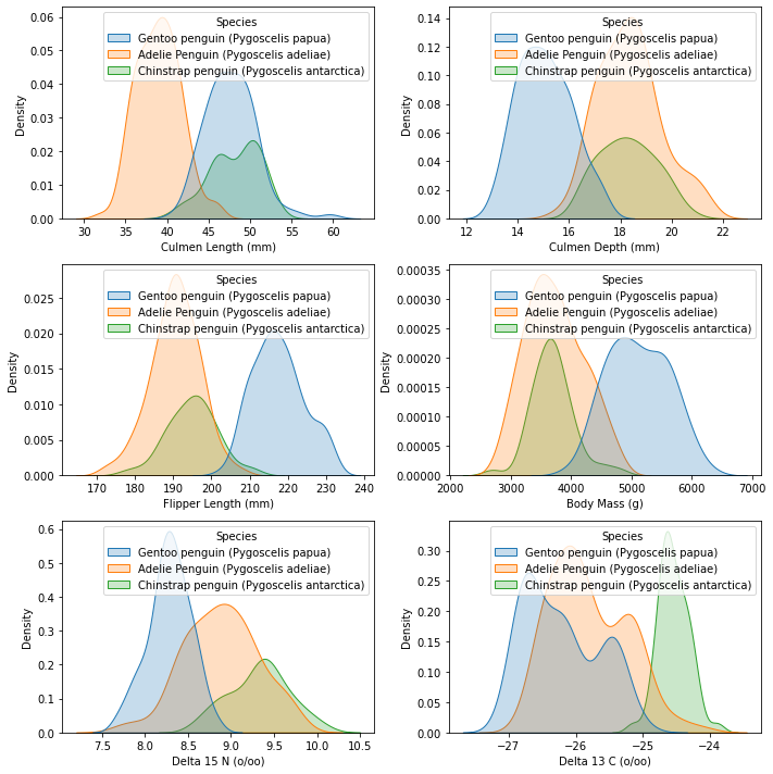
We will graph the density plots for each variable, with each line representing a different species. Density plots are useful for analyzing numerical variables; the further away the different lines are from each other, the better the predictor. In our case, if all the lines are on top of one another for a variable’s density plot, that means that the variable is similar for all the species/it isn’t very useful for distinguishing between species. Thus, it wouldn’t be a very good predictor.
def density_plot(data, m_cols, m_rows):

    '''Creates density plots for our numerical variables

    @param data: dataset to be used
    @param m_cols: number of columns
    @param m_rows: number of rows
    @return: density plot for different species based on numerical variables
    '''
    fig,ax=plt.subplots(m_rows,m_cols,figsize=(10,10))

    for k in range(len(num_vars)):

        #numerical variables in our data
        var=data[num_vars[k]]

        row=k//m_cols #the whole number part of k/m_cols (rounded towards 0)
        col=k%m_cols  #module is the remainder

        #plots density plots
        sns.kdeplot(x=var, hue=train["Species"], fill=True, ax=ax[row,col])

    #fix spacing
    plt.tight_layout()

density_plot(train, 2, 3)
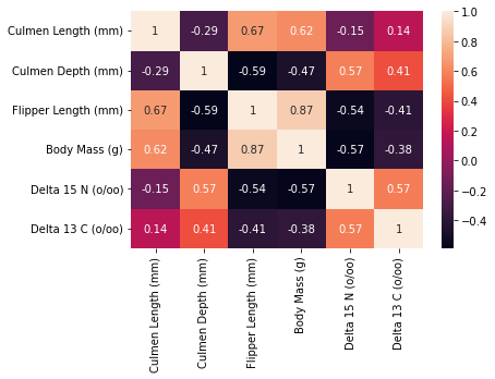
The next figure we will create to help us in analyzing/choosing our numerical variables is a correlation matrix between all of the numerical variables. Correlation matrices are useful in choosing numerical predictors; if a predictor has high correlation with another/multiple other predictors, then we should either be cautious in using it, remove it altogether, or choose between the two predictors because it means that it interacts with the other predictor(s) too much.
corrMatrix = train[num_vars].corr()

sns.heatmap(corrMatrix, annot=True)
plt.show()
Next, let’s examine our categorical variables.
train[cat_vars].head()
| Island | Clutch Completion | Sex | |
|---|---|---|---|
| 228 | Biscoe | Yes | FEMALE |
| 141 | Dream | Yes | MALE |
| 247 | Biscoe | Yes | MALE |
| 19 | Torgersen | Yes | MALE |
| 29 | Biscoe | No | MALE |
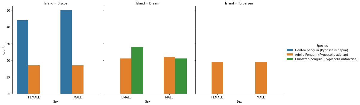
We will first examine the categorical variables “Sex” and “Island” with a figure that shows the count of each species for each gender on each island. We also include a corresponding table to verify what we see in the graphs (we include “Clutch Completion” arbitrarily so we just view one column for the count).
sns.catplot(x="Sex", hue="Species", col="Island", kind = "count", data=train, height=5, aspect=.9)
train.groupby(["Island", "Species", "Sex"])[["Clutch Completion"]].count()
| Clutch Completion | |||
|---|---|---|---|
| Island | Species | Sex | |
| Biscoe | Adelie Penguin (Pygoscelis adeliae) | FEMALE | 17 |
| MALE | 17 | ||
| Gentoo penguin (Pygoscelis papua) | FEMALE | 44 | |
| MALE | 50 | ||
| Dream | Adelie Penguin (Pygoscelis adeliae) | FEMALE | 21 |
| MALE | 22 | ||
| Chinstrap penguin (Pygoscelis antarctica) | FEMALE | 28 | |
| MALE | 21 | ||
| Torgersen | Adelie Penguin (Pygoscelis adeliae) | FEMALE | 19 |
| MALE | 19 |
We will examine our remaining categorical variable “Clutch Completion” by Species.
train.groupby(["Species", "Clutch Completion"])[["Sex"]].count()
| Sex | ||
|---|---|---|
| Species | Clutch Completion | |
| Adelie Penguin (Pygoscelis adeliae) | No | 12 |
| Yes | 103 | |
| Chinstrap penguin (Pygoscelis antarctica) | No | 9 |
| Yes | 40 | |
| Gentoo penguin (Pygoscelis papua) | No | 5 |
| Yes | 89 |
Feature Selection
We will now be selecting our final/best variables using various methods.
We’ll begin narrowing down our variables by analyzing the graphs/figures we constructed in the previous section.
For our numerical data:
In the exploratory data anlaysis section, one figure we constructed to help us in our feature selection is a correlation matrix heat map. We want to look further into the variables that have high correlation coefficients with one another (suggesting interaction effects) and decide whether we should keep the variables or choose between them. From the figure, we can see that variables with the higher correlation coefficients (>abs(0.5)) are the following:
Delta 15N and Delta 13C (0.57)
Culmen Depth and Delta 15N (0.57)
Body Mass and Flipper Length (0.87)
Culmen Length and Flipper Length (0.67)
Culmen Depth and Flipper Length (-0.59)
Delta 15N and Flipper Length (-0.54)
Body Mass and Delta 15N (-0.57)
Let’s take a further look into the variables that are highly correlated with multiple other variables: Delta 15N (3 other variables), Flipper Length (4 other variables), Culmen Depth (2 other variables), and Body Mass (2 other variables). We will be finding the p-value associated with these correlation coefficients to see if they’re statistically significant or not.
from scipy.stats.stats import pearsonr

def p_val(var1, var2):
    '''Computes correlation coefficients and corresponding p-value

    @param var1: variable
    @param var2: list of variables
    @return: correlation coefficient and corresponding p-value between var1 and variables in var2
    '''
    for i in var2:
        print("Correlation coefficient and p-value between", var1, "and", i, "is:\n", pearsonr(train[var1], train[i]))
Since the 2 variables that Body Mass and Culmen Depth are more highly correlated to are Flipper Length and Delta 15N, we will be running the function on just Flipper Length and Delta 15N
flip_vars = ["Body Mass (g)", "Culmen Length (mm)", "Culmen Depth (mm)", "Delta 15 N (o/oo)"]

p_val("Flipper Length (mm)", flip_vars)
Correlation coefficient and p-value between Flipper Length (mm) and Body Mass (g) is:
 (0.8711507498726766, 4.755275602224478e-81)
Correlation coefficient and p-value between Flipper Length (mm) and Culmen Length (mm) is:
 (0.6748080098719171, 1.2236248669331551e-35)
Correlation coefficient and p-value between Flipper Length (mm) and Culmen Depth (mm) is:
 (-0.5861548687015734, 3.355093959594431e-25)
Correlation coefficient and p-value between Flipper Length (mm) and Delta 15 N (o/oo) is:
 (-0.5416208764789054, 4.546155790880922e-21)
delta15_vars = ["Delta 13 C (o/oo)", "Body Mass (g)", "Culmen Depth (mm)"]

p_val("Delta 15 N (o/oo)", delta15_vars)
Correlation coefficient and p-value between Delta 15 N (o/oo) and Delta 13 C (o/oo) is:
 (0.5706181200230934, 1.093108387922574e-23)
Correlation coefficient and p-value between Delta 15 N (o/oo) and Body Mass (g) is:
 (-0.571199958670445, 9.625908751553983e-24)
Correlation coefficient and p-value between Delta 15 N (o/oo) and Culmen Depth (mm) is:
 (0.5746830815407217, 4.472629961782847e-24)
As we can see from running the above function to find the p-values associated with the correlation coefficients, since they all have siignificantly small p-values, they’re are significantly significant. However, that doesn’t mean we should remove all of these variables; we need to take into account the value of the correlation cofficients, how many other variables they’re more highly correlated with, and their density plots.
Since Body Mass and Culmen Depth are only more highly correlated with 2 other variables (Flipper Length and Delta 15N), and the variables they’re correlated with are highly correlated with 3/4 other variables, we will focus on the 2 variables (Flipper Length and Delta 15N) (since, if we do remove these two variables, Body Mass and Culmen Depth will be fine because they’re no longer highly correlated with another variable).
We’ll begin with Flipper Length. As we can see from the correlation matrix, not only does Flipper Length have the highest correlation coefficients out of any other variable, but it is also highly correlated with the most amount of variables (4)! This suggests that we should remove Flipper Length because removing it may significantly decrease interaction effects between variables. However, before we decide to remove it, let’s take a look at our density plot for Flipper Length that was constructed in the previous section. Looking at the plot, we can see that Flipper Length could potentially be useful in distinguishing Gentoo from Adelie and Chinstrap. However, Culmen Depth’s density plot suggests that it can also do the same and, unlike Flipper Length, without the added threat of high correlation coefficients/interaction effects. Thus, we will remove Flipper Length as a contender for our final numerical predictors.
Next, let’s examine Delta 15N. The correlation coefficients for Delta 15N aren’t as high the ones for Flipper Length, but they are still on the higher side (~abs(0.54-0.58)) and it is highly correlated with 3 other variables. Let’s take a look at its density plot. Its density plot is not convincing enough for us to keep it; in addition to the fact that Delta 15N is more highly correlated with 3 other variables, the densities are too close to each other/on top of one another to convince us that it’s a good predictor. Thus, we will also remove Delta 15N as a contender for our final numerical predictors.
Since we removed Flipper Length and Delta 15N, Body Mass and Culmen Depth are no longer highly correlated with the other final numerical predictor contenders and thus are still in the running.
Our current contenders are Body Mass, Culmen Depth, Culmen Length, and Delta 13C. From the density plots, it appears that Culmen Depth and Culmen Length may be our best numerical predictors, but we will use logistic regression to verify this after we choose our final categorical predictor contenders.
For our categorical data:
The categorical data we analyzed in the exploratory data analysis section includes the variables Sex, Island, and Clutch Completion.
To analyze the significance of Sex and Island, we constructed side-by-side bar charts to help us see the amount of female and male penguins by species by island and a corresponding table to verify the results of our figure. From the figure, we can see that each Island has a different mixture of species: Biscoe has Adelie and Gentoo (though, there’s significantly more Gentoo), Dream has Adelie and Chinstrap, and Torgersen only has Adelie. This observation suggests that Island may be a good predictor; for example, if our penguin is on Torgersen, it’s most likely of the species Adelie. The figure also suggests that Sex may be a bad predictor; there is about a 50/50 ratio of female to male penguins on each Island for each Species. This observation is further backed up by the corresponding table we constructed that showcases the amount of females and males for each species on each island. Thus, we will remove Sex as a final categorical variable contender.
We are left with Clutch Completion and Island. We already discussed how Island has the potential to be a good categorical predictor, so now we’ll focus on Clutch Completion. For this variable, we constructed a table that showcases the amount of Yes and No’s per species. Since we do not have the same amount of penguins for each species, we will calculate the proportion of Yes’s per species from the table.
print("Proportion of Adelie that reached Clutch Completion:", round(103/(103+12),3))
print("Proportion of Gentoo that reached Clutch Completion:", round(40/(40+9),3))
print("Proportion of Chinstrap that reached Clutch Completion:", round(89/(89+5),3))
Proportion of Adelie that reached Clutch Completion: 0.896
Proportion of Gentoo that reached Clutch Completion: 0.816
Proportion of Chinstrap that reached Clutch Completion: 0.947
As we can see, the proportion of Yes’s per species are all within 0.131 from each other. Since these differences aren’t super close to one another and we’re not sure if these differences are significant or not, we’ll move onto using logistic regression to select our final categorical predictor and numerical predictors by testing each combination and computing and comparing the training and testing scores.
from sklearn.linear_model import LogisticRegression
from sklearn.model_selection import cross_val_score
from sklearn import preprocessing
le=preprocessing.LabelEncoder()

X_train["Island"]=le.fit_transform(X_train["Island"])
X_train["Clutch Completion"]=le.fit_transform(X_train["Clutch Completion"])

LR=LogisticRegression(max_iter = 500)

def check_column_score(cols):
    """Trains and evaluates  a model via cross validation on the columns of the data
    with selected indices

    @param cols: list of columns/variables
    @return: cross validation score
    """

    print("training with columns" + str(cols))
    return cross_val_score(LR,X_train[cols],y_train.values,cv=5).mean()

combos = [['Island', 'Culmen Length (mm)', 'Culmen Depth (mm)'],
          ['Island', 'Culmen Length (mm)', 'Body Mass (g)'],
          ['Island', 'Culmen Depth (mm)', 'Body Mass (g)'],
          ['Clutch Completion', 'Culmen Length (mm)', 'Culmen Depth (mm)'],
          ['Clutch Completion', 'Culmen Length (mm)', 'Body Mass (g)'],
          ['Clutch Completion', 'Culmen Depth (mm)', 'Body Mass (g)']]


for combo in combos:
    x=check_column_score(combo)
    print("CV score is "+ str(np.round(x,3)))
training with columns['Island', 'Culmen Length (mm)', 'Culmen Depth (mm)']
CV score is 0.973
training with columns['Island', 'Culmen Length (mm)', 'Body Mass (g)']
CV score is 0.969
training with columns['Island', 'Culmen Depth (mm)', 'Body Mass (g)']
CV score is 0.81
training with columns['Clutch Completion', 'Culmen Length (mm)', 'Culmen Depth (mm)']
CV score is 0.957
training with columns['Clutch Completion', 'Culmen Length (mm)', 'Body Mass (g)']
CV score is 0.934
training with columns['Clutch Completion', 'Culmen Depth (mm)', 'Body Mass (g)']
CV score is 0.81
#check with test set:
X_test["Island"]=le.fit_transform(X_test["Island"])
X_test["Clutch Completion"]=le.fit_transform(X_test["Clutch Completion"])

def test_column_score(cols):
    """Test the performance of the model trained on the columns of the data
    with selected indeces

    @param cols: list columns/of variables
    @return: cross validation score
    """

    print("training with columns" + str(cols))
    LR=LogisticRegression(max_iter=500)
    LR.fit(X_train[cols],y_train)

    return LR.score(X_test[cols],y_test)

for cols in combos:
    x=test_column_score(cols)
    print("The test score is " + str(np.round(x,3)))
training with columns['Island', 'Culmen Length (mm)', 'Culmen Depth (mm)']
The test score is 0.985
training with columns['Island', 'Culmen Length (mm)', 'Body Mass (g)']
The test score is 0.97
training with columns['Island', 'Culmen Depth (mm)', 'Body Mass (g)']
The test score is 0.727
training with columns['Clutch Completion', 'Culmen Length (mm)', 'Culmen Depth (mm)']
The test score is 0.955
training with columns['Clutch Completion', 'Culmen Length (mm)', 'Body Mass (g)']
The test score is 0.97
training with columns['Clutch Completion', 'Culmen Depth (mm)', 'Body Mass (g)']
The test score is 0.727
Our logistic regression model suggests that, out of our final contenders, Island, Culmen Length (mm), and Culmen Depth (mm) are best predictors because they had both the highest training and test scores. The training and testing scores are also pretty close, which suggests that overfitting is not an issue in this model. Thus, we will construct our models with these 3 variables as our predictors.
Modeling
Now that we have our final predictors, we’ll move onto modeling. We will try 3 different machine learning models: Support Vector Machine, KNN Nearest Neighbors, and Random Forest.
Let’s begin by encoding our final categorical variable and creating a vector of our final variables.
from sklearn import preprocessing

final_vars = ["Island", "Culmen Length (mm)", "Culmen Depth (mm)"]

le = preprocessing.LabelEncoder()
X_train["Island"] = le.fit_transform(X_train["Island"])
X_test["Island"] = le.fit_transform(X_test["Island"])

#encoded y_test for decision region plots
y_test_dc = le.fit_transform(y_test)
def plot_regions(c,X,y):
    '''Creates graphs with decision regions corresponding to model

    @param c: machine learning model
    @param X: predictor variable
    @param y: target variable
    @return: Graph with decision regions corresponding to model and data
    '''

    c.fit(X,y)

    x0=X["Culmen Length (mm)"]
    x1=X["Culmen Depth (mm)"]

    grid_x=np.linspace(x0.min(),x0.max(),501)
    grid_y=np.linspace(x1.min(),x1.max(),501)

    xx,yy=np.meshgrid(grid_x,grid_y)
    np.shape(xx),np.shape(yy)

    XX=xx.ravel()
    YY=yy.ravel()

    #np.shape(np.c_[XX,YY])

    p=c.predict(np.c_[XX,YY])

    p=p.reshape(xx.shape)

    fig,ax=plt.subplots(1)

    #plot the decision regions
    ax.contourf(xx,yy,p,cmap="jet",alpha=.2)

    ax.scatter(x0,x1,c=y,cmap="jet")

    ax.set(xlabel="Culmen Length (mm)",ylabel="Culmen Depth (mm)")
Support Vector Machine
We will be constructing a Support Vector Machine model and the parameter we will be choosing with cross validation is C (regularization parameter). Seeing as how well the testing data scored from our logistic regression model (which usually has a linear decision boundary) in our feature selection, we will be using a linear kernel (which has linear decision boundaries).
from sklearn import svm
from sklearn.model_selection import cross_val_score
#cross-validation to find our best C
best_score=-np.inf
N=30 #largest max C
scores=np.zeros(N)
for d in range(1,N+1):
SVM=svm.SVC(kernel="linear", C=d, random_state=1128)
scores[d-1]=cross_val_score(SVM,X_train[final_vars],y_train,cv=10).mean()
if scores[d-1]>best_score:
best_C=d
best_score=scores[d-1]
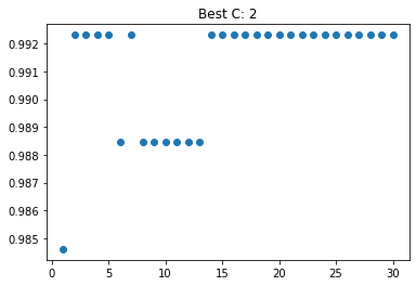
best_C, best_score
(2, 0.9923076923076923)
As we can see from the above code, our best C is 2, with a cross validation score of about 0.99. From the graoph below, we can see that once our C nears 5, it levels off, but before that, 2 has about the same score.
def best_graph(N, scores, best_val, param):
    '''Creates graph of values and corresponding scores

    @param N: largest max value
    @param scores: cross validation scores
    @param best_val: best value from cross validation
    @param param: parameter we're getting best value for
    @return: graph of values and corresponding scores
    '''
    fig,ax=plt.subplots(1)
    ax.scatter(np.arange(1,N+1),scores)
    ax.set(title="Best "+param+": "+str(best_val))

best_graph(N,scores,best_C,"C")
We will now construct our Support Vector Machine Model with our best C, fit it to our training set with our final variables, and construct the corresponding confusion matrix and testing score when we test it against our testing set.
from sklearn.metrics import confusion_matrix
#construct SVM model
SVM=svm.SVC(kernel="linear", C=best_C, random_state=1128)

#fit model to training set, but only with our final chosen variables
model=SVM.fit(X_train[final_vars], y_train)

#predict using testing set and construct corresponding confusion matrix
y_test_pred=model.predict(X_test[final_vars])
y_test_pred

c=confusion_matrix(y_test,y_test_pred)
c, model.score(X_test[final_vars], y_test)
(array([[23,  1,  0],
        [ 0, 18,  0],
        [ 0,  0, 24]]),
 0.9848484848484849)
We get a testing score of about 0.985, where the model only guessed incorrectly once!
Decision Region:
Let’s examine the decision region plot between our final variables Culmen Length and Culmen Depth by species
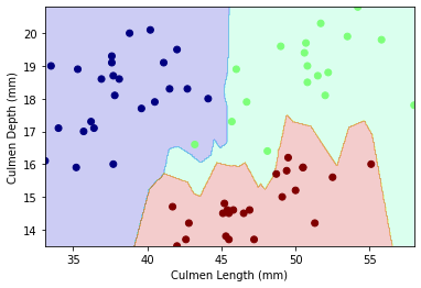
plot_regions(SVM,X_test[["Culmen Length (mm)","Culmen Depth (mm)"]],y_test_dc)
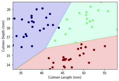
Our decision region plot supports our confusion matrix: there only seems to be 1 wrong guess! Our decision boundary for this model is linear.
Random Forest
Next, we will be constructing a model using Random Forest and the parameter we’re choosing using cross validation is n_estimators (number of trees in the forest).
from sklearn.ensemble import RandomForestClassifier

#cross validation for n_estimators
best_score=0
Ns=[10,50,100,250,500]

for n in Ns:
    F=RandomForestClassifier(n_estimators=n, random_state = 1128)
    cvs=cross_val_score(F,X_train[final_vars],y_train,cv=10).mean()
    if cvs>best_score:
        best_n=n
        best_score=cvs

print(best_n)
print(best_score)
10
0.9806153846153848
From cross validation, our best n_estimator is 10 with a cross validation score of about 0.981.
We will now be constructing our Random Forest Classifier model with our best n, fitting it to our training set with our final variables, and constructing the corresponding confusion matrix and testing score when we test it against our testing set.
m = RandomForestClassifier(best_n, random_state=1128)
model2 = m.fit(X_train[final_vars],y_train)

#confusion matrix
y_test_pred=model2.predict(X_test[final_vars])

c=confusion_matrix(y_test,y_test_pred)
c, model2.score(X_test[final_vars], y_test)
(array([[23,  0,  1],
        [ 0, 18,  0],
        [ 2,  0, 22]]),
 0.9545454545454546)
We get a testing score of about 0.955, where the model guessed incorrectly 3 times. This model performed worse than our Support Vector Machine model.
Decision Region:
Let’s examine the decision region plot between our final variables Culmen Length and Culmen Depth by species
plot_regions(m,X_test[["Culmen Length (mm)","Culmen Depth (mm)"]],y_test_dc)
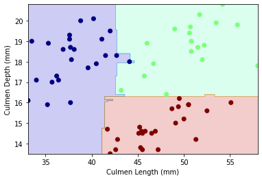
The decision boundary for this model is non-linear.
KNN Nearest Neighbors
The final model we will be constructing is a KNN model, and we will be using cross validation to find the best n_neighbors.
from sklearn.neighbors import KNeighborsClassifier

#cross-validation to find our best C
best_score=-np.inf
N=40 #largest max n_neighbors
scores=np.zeros(N)

for i in range(1,N+1):
    knn = KNeighborsClassifier(n_neighbors=i)
    scores[i-1]=cross_val_score(knn,X_train[final_vars],y_train,cv=10).mean()
    if scores[i-1]>best_score:
        best_nn=i
        best_score=scores[i-1]

best_nn, best_score
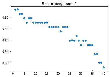
(2, 0.976923076923077)
From cross validation, our best n_neighbors is 2 with a cross validation score of about 0.977. The graph we constructed below supports this: the n_neighbors value with the highest score does appear to be 2.
best_graph(N,scores,best_nn,"n_neighbors")
Now that we have our best parameter value, we will now construct our KNN model with the value, fit it to our training set with our final variables, and construct the corresponding confusion matrix and testing score when we test it against our testing set.
knn = KNeighborsClassifier(n_neighbors=best_nn)

knn.fit(X_train[final_vars],y_train)

#confusion matrix
y_test_pred=knn.predict(X_test[final_vars])

c=confusion_matrix(y_test,y_test_pred)
c, knn.score(X_test[final_vars], y_test)
(array([[24,  0,  0],
        [ 0, 17,  1],
        [ 0,  0, 24]]),
 0.9848484848484849)
We get a testing score of about 0.985, where the model only guessed incorrectly once! This model performed just as well as the Support Vector Machine.
Decision Region:
Let’s examine the decision region plot between our final variables Culmen Length and Culmen Depth by species
plot_regions(knn,X_test[["Culmen Length (mm)","Culmen Depth (mm)"]],y_test_dc)
Our decision region plot supports our confusion matrix: there only seems to be 1 wrong guess! Our decision boundary for this model is non-linear.
Summary
Based on the exploratory data analysis, feature selection, and modeling, I suggest that the best combination of models and features is the Support Vector Machine model with a C value of 2 and variables Culmen Length, Culmen Depth, and Island.
In terms of the models themselves, SVM and KNN performed equally well, each scoring a testing score of about 0.985 with only 1 wrong guess. However, I decided to choose SVM because it gets the same job done without being too complex, and thus is more efficient. The third model, the random forest classifier, performed the worst, with a testing score of about 0.955 and 3 wrong guesses. I believe these mistakes made by the models may be due to the fact that some of the data points for the different species are very close to one another and thus may be mistakenly classified.
I believe that, if more data was available, KNN would end up performing better than SVM because of the fact that it has a non-linear decision boundary, which may be more helpful for more complex data. However, I believe that if we had different data in which the data points for each species are more clustered together, SVM would make less mistakes.