Introduction

This page contains the final project for my Introduction to Statistical Models and Data Mining class in Fall 2021.

Abstract

This Kaggle project aims to predict the diagnosis of heart disease using statistical learning models based on the training and testing data sets provided. This paper provides a clear description of how we built the final model, including introduction, data analysis & cleaning, feature selection, methodology, and conclusions and limitations.

The final model is a logistic regression with a misclassification rate of 0.1893365 and a Kaggle score of 0.80869. The model used four numerical and seven categorical predictors: Cholesterol, MaxHR, Oldpeak, avg_glucose_level, Sex, FastingBS, RestingECG, ExerciseAngina, ever_married, work_type, Residence_type, and stroke.

Introduction

Heart disease is a significant and lethal issue that, according to the World Health Organization, causes an estimated 12 million deaths worldwide each year (Krishnaiah V. et al.). Due to the prevalence of heart disease, early and accurate diagnoses are integral to its prevention. In fact, early and accurate diagnoses of coronary heart disease, one of the most common diseases in the world, helps reduce mortality rates by allowing for appropriate and early treatment of the condition (Abdar M. et al.). Not only can these diagnoses prevent deaths, but they can also eradicate unnecessary hospital costs. After all, heart disease contributed to 31% of the $30.8 billion in potentially preventable hospital costs in 2006 (Dai W. et al.). One of the proposed solutions to providing more reliable diagnoses for heart disease is through data mining and data machines techniques, which could potentially reduce the time it takes for a diagnosis and increase the accuracy (Krishnaiah V. et al.).

In this Kaggle project, we utilized various data mining techniques, such as data cleaning and building machine learning models to predict the existence of heart disease from various predictors related to heart disease. We used a training dataset, which included the target variable HeartDisease to construct models to predict the target variable diagnosis “Yes” or “No” in our testing dataset.

Data Analysis, Cleaning & Imputation

Data Set Overview

We were provided with two data sets to conduct our analysis, one for testing and one for training. The training data set contained seven numerical variables and thirteen categorical, one of the categorical variables was our response variable HeartDisease. The testing data set contained the same seven numerical variables and twelve categorical variables because it excluded the response variable. The numerical variables included Age, RestingBP, Cholesterol, MaxHR, Oldpeak, avg_glucose_level, and bmi, while the categorical variables included Sex, ChestPainType, FastingBS, RestingECG, ExerciseAngina, ST_slope, hypertension, ever_married, work_type, Residence_type, smoking_status, stroke, and HeartDisease. Furthermore, the training data set had 4220 observations and the testing had 1808 observations.

library(readr)
HDtrainNew <- read_csv("/Users/k/Documents/STATS 101C/Data sets/HDtrainNew.csv")
HDtestNoYNew <- read_csv("/Users/k/Documents/STATS 101C/Data sets/HDtestNoYNew.csv")

HDtrain <- HDtrainNew[,-1]
HDtest <- HDtestNoYNew[,-1]

dim(HDtrain)
dim(HDtest)

#Numerical and categorical variables

num_train <- HDtrain[sapply(HDtrain,is.numeric)]
length(num_train) 

num_test <- HDtest[sapply(HDtest,is.numeric)]
length(num_test)

#7 numerical variables in both training and testing data; thus, there are 13 categorical variables in both the training and testing data 

Data Cleaning

The first step of our data cleaning process was turning categorical predictors of type ‘character’ into factors. To do this, we had to manipulate some of the variables so that the levels of the training and testing data set matched. The Sex variable had a mix of “F”, “M”, “Female”, and “Male,” so we changed all the “F” into “Female” and all the “M” into “Male” in both data sets. The variable smoking_status had missing values and a level “Unknown”. Since we are assuming these NA values are missing completely at random, we changed the NA values in the variable to “Unknown”.

#turn training data categorical predictors into factors
HDtrain[sapply(HDtrain,is.character)] <- lapply(HDtrain[sapply(HDtrain,is.character)], factor)

#turn testing data categorical predictors into factors
HDtest[sapply(HDtest,is.character)] <- lapply(HDtest[sapply(HDtest,is.character)], factor)

#clean up Sex variable so they all match
HDtrain[which(HDtrain$Sex == 'F'),1] = 'Female'
HDtrain[which(HDtrain$Sex == 'M'),1] = 'Male'

HDtest[which(HDtest$Sex == 'F'),1] = 'Female'
HDtest[which(HDtest$Sex == 'M'),1] = 'Male'

#change missing values in smoking_status to "Unknown"
HDtrain$smoking_status[is.na(HDtrain$smoking_status)] <- "Unknown"
HDtest$smoking_status[is.na(HDtest$smoking_status)] <- "Unknown"

#Training: missing values
length(HDtrain[is.na(HDtrain)==TRUE])
#about 1893 missing values

#Testing: missing values
length(HDtest[is.na(HDtest)==TRUE])
#about 1148 missing values

library(VIM)

HDtraintNA_plot <- aggr(HDtrain, col=c('blue','green'),
numbers=TRUE, sortVars=TRUE, labels=names(HDtrain), cex.axis=.7, gap=3, ylab=c("Missing data","Pattern"))
#ever_married, work_type, residence_type; each has 631 missing values and each accounts for 14.95261% of the total data for each variable

HDtestNA_plot <- aggr(HDtest, col=c('blue','green'),
numbers=TRUE, sortVars=TRUE, labels=names(HDtest), cex.axis=.7, gap=3, ylab=c("Missing data","Pattern"))
#ever_married, work_type, residence_type; each has 287 missing values and each accounts for 15.87389% of the total data for each variable 

Data Imputation

The next step of our data cleaning process was dealing with the missing values in our dataset. Although we initially had 4 variables with missing values, after changing the missing values in smoking_status to “Unknown,” we were left with 3: ever_married, work_type, and Residence_type. After some analysis, we discovered that we had about 1893 total missing values in our training data and 1148 missing values in our testing data. In the training data, each variable had 631 missing values, which accounted for 14.95261% of the total data for each variable, while in the testing data, each variable had 287 missing values, accounting for 15.87389% of the total data for each variable. To deal with these missing values, we decided to use the MICE package in R to impute them.

After perusing through the various methods included in the MICE package, we decided to try three different methods: default (logreg and polyreg), pmm (predictive means matching), and sample. We ran the imputations using each method and created new datasets with them, then compared the proportion tables for each variable to see which method came closest to our original data. We found that the sample method came closest to the original data for both ever_married and work_type, while pmm came closest to the original data for Residence_type. Thus, we decided to use the sample method in MICE to impute the training and testing data.

 
 #Let's impute our missing values. We'll try with the default methods, pmm, and sample

library(mice)

HDtrainMICE <- mice(HDtrain, m=1, seed = 1128,  defaultMethod = c("pmm", "logreg", "polyreg", "polr"))
summary(HDtrainMICE)
HDtrainMICE.data <- complete(HDtrainMICE)

HDtrainMICE.pmm<- mice(HDtrain, m=1, method = 'pmm', seed = 1128)
summary(HDtrainMICE.pmm)
HDtrainMICE.pmm.data <- complete(HDtrainMICE.pmm)

HDtrainMICE.samp <- mice(HDtrain, m=1, method = 'sample', seed = 1128)
HDtrainMICE.samp.data <- complete(HDtrainMICE.samp)

prop.table(table(HDtrain$ever_married))
prop.table(table(HDtrainMICE.data$ever_married))
prop.table(table(HDtrainMICE.pmm.data$ever_married))
prop.table(table(HDtrainMICE.samp.data$ever_married))
#sample.data is closest to OG data for ever_married

prop.table(table(HDtrain$work_type))
prop.table(table(HDtrainMICE.data$work_type))
prop.table(table(HDtrainMICE.pmm.data$work_type))
prop.table(table(HDtrainMICE.samp.data$work_type))
#sample.data is closest to OG data for work_type

prop.table(table(HDtrain$Residence_type))
prop.table(table(HDtrainMICE.data$Residence_type))
prop.table(table(HDtrainMICE.pmm.data$Residence_type))
prop.table(table(HDtrainMICE.samp.data$Residence_type))
#pmm is closest to OG data for Residence_type

#we will use the imputations using the sample method, since it matches the original data best

##imputing test data 

HDtestMICE.samp <- mice(HDtest, m=1, method = 'sample', seed = 1128)
HDtestMICE.samp.data <- complete(HDtestMICE.samp)

Exploratory Data Analysis and Variable Selection

We analyzed the variables provided to us using exploratory data analysis to better understand their significance in accurately predicting our target variable to choose the “best” ones. Through prior knowledge and research, we learned that various factors, such as ECG, blood pressure, cholesterol, and blood sugar (Khourdifi Y. et al.) are known to impact and detect heart disease, so we kept these variables in mind.

Variable Selection/EDA: Numerical Variables

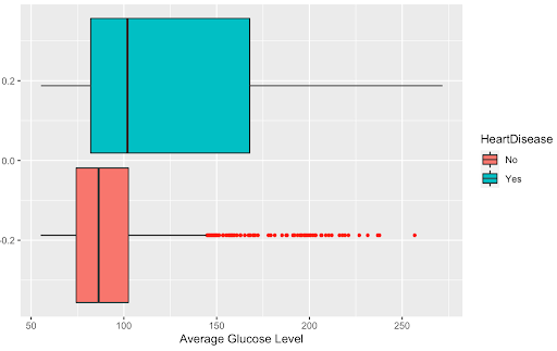
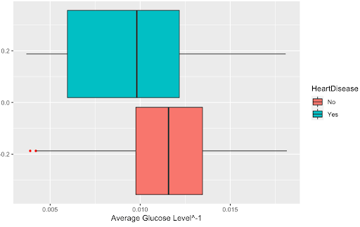
First, we transformed each of our numerical variables and analyzed whether this transformation was beneficial. After examining a boxplot of all our numerical variables and whether the transformation helped the distribution, we found that only transformation was beneficial to the variable: the inverse of avg_glucose_level. Below are the boxplots of the variable before and after it was transformed to show that the transformation.

##Numerical predictors

## Transformations and Boxplots for Numerical Variables

library(car)
powerTransform(HDtrain$avg_glucose_level)
powerTransform(HDtrain$bmi)
powerTransform(HDtrain$Age)
powerTransform(HDtrain$MaxHR)

For our numerical variables, we chose which to use by analyzing the density plots and by creating a correlation matrix. Since the response variable is binary, we analyzed the density plots to identify which numerical variables had clear differences in their distribution. Those which did have a clear difference were kept as potential significant predictors to use in our models, while those that did not have a clear difference were no longer considered for our model.

## Correlation matrix 

library(Hmisc)
rcorr(as.matrix(HDtrain[,sapply(HDtrain,is.numeric)]))

#highest correlation coefficients w/ significant p-values: Age&MaxHR, avg_glucose_level&Cholesterol, so we will be careful with these variables when constructing our models

#plotting densities of numerical variables
g1 <- ggplot(HDtrain, aes(x=Age, color = HeartDisease)) + geom_density()
g2 <- ggplot(HDtrain, aes(x=RestingBP, color = HeartDisease)) + geom_density()
g3 <- ggplot(HDtrain, aes(x=Cholesterol, color = HeartDisease)) + geom_density()
g4 <- ggplot(HDtrain, aes(x=MaxHR, color = HeartDisease)) + geom_density()
g5 <- ggplot(HDtrain, aes(x=Oldpeak, color = HeartDisease)) + geom_density()
g6 <- ggplot(HDtrain, aes(x=avg_glucose_level, color = HeartDisease)) + geom_density()
g7 <- ggplot(HDtrain, aes(x=bmi, color = HeartDisease)) + geom_density()

library(gridExtra) 
grid.arrange(g1,g2,g3,g4,nrow=2)
grid.arrange(g5,g6,g7,nrow=2)

#the graphs seem to suggest that avg_glucose_level, Age, and MaxHR are good numerical predictors

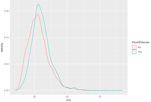
Shown below is the density plot of the bmi variable. This density plot is an example of a variable with no clear difference in distribution; so, it was not considered for our models.

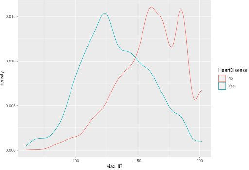
Shown below is the density plot of the max heart rate (MaxHR) variable. This density plot is an example of a variable with a clear difference in distribution; so, it was considered for our models.

From our density plots, the numerical variables that are potentially significant are Age, MaxHR, Oldpeak, avg_glucose_level, and Cholesterol.

Additionally, we found correlations and p-values between all the numerical variables. If two variables have a p-value less than 0.05 then their correlation is significant and need to proceed with caution if using both variables in our model. The highest correlation coefficients with significant p-values are Age with MaxHR and avg_glucose_level with Cholesterol. Age and MaxHR had a correlation of -0.69 while avg_glucose_level and Cholesterol had a correlation of -0.78. Since these variables had the greatest significant correlation with one another we ran logistic models to see the importance of the variables. We ran a total of three different logistic models for each pairing: two of the models with each respective variable in the pair by itself and one model with the pair together. The three models using Age and MaxHR told us that, by looking at the AIC, it is a lot more beneficial to just use MaxHR. The three models using avg_glucose_level and Cholesterol told us that, by looking at the AIC, avg_glucose_level is the more beneficial of the two variables to use, but since the AIC didn’t change by much across the models, we could potentially include them together. We will keep these findings in mind when creating our final model.

 
summary(glm(HeartDisease~Age, family=binomial, data=HDtrain))
summary(glm(HeartDisease~MaxHR, family=binomial, data=HDtrain))
summary(glm(HeartDisease~MaxHR+Age, family=binomial, data=HDtrain))
#by looking at AIC, we can see that the model with just MaxHR is better (and by a lot), so we will keep that in mind

summary(glm(HeartDisease~avg_glucose_level, family=binomial, data=HDtrain))
summary(glm(HeartDisease~Cholesterol, family=binomial, data=HDtrain))
summary(glm(HeartDisease~avg_glucose_level+Cholesterol, family=binomial, data=HDtrain))
#avg_glucose_level seems to have a better model (though not by too much) so we will keep that in mind
 

The final step in our variable selection process was to perform stepwise logistic regression on the numerical variables alone. Since our earlier analysis of our numerical predictors suggested that a transformed avg_glucose_level could be beneficial, for our numerical predictors, we decided to run two stepwise logistic regressions: one with the original avg_glucose_level predictor and one with a transformed avg_glucose_level called newglucose. For our stepwise logistic regression models, we first ran two simple logistic regression models with each glucose variable and calculated the variance inflation factor. Since the VIF for each variable was less than 5 in both models, we continued with the stepwise selection, where we used the function stepAIC with an exhaustive method. The stepwise logistic regression model with the original avg_glucose_level chose Cholesterol, MaxHR, OldPeak, and avg_glucose_level. This validates our earlier analysis that MaxHR is a good predictor and should be chosen over Age. This also validates our earlier analysis that avg_glucose_level would be a good numerical predictor and that, while removing Cholesterol did improve the AIC value, it was not improved by much, so having Cholesterol and avg_glucose_level together is not as drastic as having MaxHR and Age together. The stepwise logistic regression model with newglucose chose Cholesterol, MaxHR, Oldpeak, newglucose, and bmi.

 
## Logistic Regression

##We will run a stepwise selection model with a combination of forward and backwards selection with our numerical variables to choose the best variables


#since the transformations from earlier suggested that transformation avg_glucose_level could be beneficial, we will run two stepwise selections: one with the original avg_glucose_level and one with a new variable: newglucose, which the the transformed avg_glucose_level
HDtrainMICE.samp.data$newglucose <- (HDtrainMICE.samp.data$avg_glucose_level)^-1

library(car)
library(MASS)

#model with original glucose
testing <-  glm(HeartDisease ~ RestingBP+Cholesterol+MaxHR+Oldpeak+avg_glucose_level+bmi+Age, family = binomial, data = HDtrainMICE.samp.data)

#model with transformed glucose variable
testing.ng <-  glm(HeartDisease ~ RestingBP+Cholesterol+MaxHR+Oldpeak+newglucose+bmi+Age, family = binomial, data = HDtrainMICE.samp.data)

vif(testing) #values < 5

vif(testing.ng) #values < 5

testing.step <- stepAIC(testing, method = "exhaustive", trace=F)
testing.step.ng <- stepAIC(testing.ng, method = "exhaustive", trace=F)

#the first step model chose: Cholesterol, MaxHR, OldPeak, and avg_glucose_level; this validates our earlier analysis that MaxHR is a good predictor and should be chosen over Age. This also validates our earlier analysis that avg_glucose_level would be a good numerical predictor and that, while removing Cholesterol did improve the AIC value, it was not improved by much so having Cholesterol and avg_glucose_level together is not as drastic as having MaxHR and Age together

#the step model with the transformed glucose chose: Cholesterol, MaxHR, Oldpeak, newglucose, and bmi

Variable Selection/EDA: Categorical Variables

For each categorical variable, we first ran a Chi-Squared Test and analyzed which variables had a significant p-value. Each test was built between the HeartDisease variable and a categorical variable.

##Categorical predictors

ChiSquareTest <- function(x){
  test <- chisq.test(x, HDtrain$HeartDisease)
  return(test$p.value)
}

lapply(HDtrain[,sapply(HDtrain,is.factor)], ChiSquareTest)

#variables with significant p-values: Sex, ChestPainType, ExerciseAngina, ST_slope, FastingBS, hypertension, ever_married, work_type, smoking_status, stroke

p-value

p-value Sex 1.78417e-07 hypertension 1.737685e-42 ChestPainType 0.0004421053 ever_married 9.771532e-67 FastingBS 1.00708e-0.83 work_type 4.351961e-48 RestingECG 0.2634605 Residence_type 0.07837005 ExerciseAngina 7.843483e-09 smoking_status 3.966361e-11 ST_slope 1.127634e-06 stroke 2.86475e-25

After conducting the Chi-Squared Tests, we found that categorical variables with a significant p-value (<0.05) are the following: Sex, ChestPainType, ExerciseAngina, ST_slope, FastingBS, hypertension, ever_married, work_type, smoking_status, and stroke. This means there is a strong causal relationship between these categorical variables and HeartDisease.

Furthermore, for each categorical variable, we plotted bar graphs separated by the binary response variable, HeartDisease, to see which variables had distinct different distributions. We found that the bar graphs indicated that stroke, ever_married, work_type, hypertension, FastingBS, and smoking_status were all significant predictors while the rest were not. Since these variables were also significant in our chi-squared test, they were chosen as the potential categorical predictors that we were to use going forward.

library(ggplot2)
c1 <- ggplot(HDtrain,aes(Sex,fill=HeartDisease))+geom_bar()
c2 <- ggplot(HDtrain,aes(ChestPainType,fill=HeartDisease))+geom_bar()
c3 <- ggplot(HDtrain,aes(ExerciseAngina,fill=HeartDisease))+geom_bar()
c4 <- ggplot(HDtrain,aes(ST_Slope,fill=HeartDisease))+geom_bar()
c5 <- ggplot(HDtrain,aes(FastingBS,fill=HeartDisease))+geom_bar()
c6 <- ggplot(HDtrain,aes(hypertension,fill=HeartDisease))+geom_bar()
c7 <- ggplot(HDtrainMICE.samp.data,aes(ever_married,fill=HeartDisease))+geom_bar()
c8 <- ggplot(HDtrainMICE.samp.data,aes(work_type,fill=HeartDisease))+geom_bar()
c9 <- ggplot(HDtrain,aes(smoking_status,fill=HeartDisease))+geom_bar()
c10 <- ggplot(HDtrain,aes(stroke,fill=HeartDisease))+geom_bar()
c11 <- ggplot(HDtrain,aes(RestingECG,fill=HeartDisease))+geom_bar()
c12 <- ggplot(HDtrainMICE.samp.data,aes(Residence_type,fill=HeartDisease))+geom_bar()

grid.arrange(c1,c2,c3,c4, nrow=2)
grid.arrange(c5,c6,c7,c8, nrow=2)
grid.arrange(c9,c10,c11,c12, nrow=2)

#graphs suggest that significant predictors seem to be: stroke, ever_married, work_type, hypertension, FastingBS, smoking_status, which are all also significant in the chi-square test

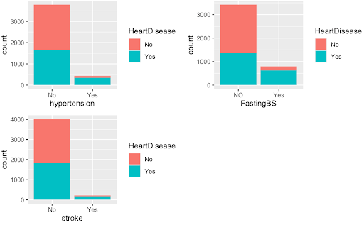
The graphs above on the top are examples of the variables we found were significant predictors while the graphs on the bottom were examples of variables we deemed as poor predictors of the HeartDisease variable.

Next, we performed stepwise logistic regression on the categorical variables alone to choose our predictors. We first ran a logistic regression model with all of our categorical predictors and calculated the VIF. Since the variables ST_slope and ChestPainType had VIF values greater than 5, we decided to remove them and run a logistic regression model without them. We then used stepAIC with the exhaustive method, which ended up choosing Sex, FastingBS, RestingECG, ExerciseAngina, ever_married, work_type, Residence_type, and stroke This validates our earlier analysis with the chi-square test and bar graphs that stroke, ever_married, work_type, and FastingBS could be good categorical predictors.

##We will run a stepwise selection model with a combination of forward and backwards selection with our categorical variables to choose the best variables

testing2 <-  glm(HeartDisease ~ .-(RestingBP+Cholesterol+MaxHR+Oldpeak+avg_glucose_level+bmi+Age), family = binomial, data = HDtrainMICE.samp.data)

vif(testing2) #ST_slope and ChestPainType have high values, so let's remove them

testing2 <-  glm(HeartDisease ~ .-(RestingBP+Cholesterol+MaxHR+Oldpeak+avg_glucose_level+bmi+Age+ChestPainType+ST_Slope), family = binomial, data = HDtrainMICE.samp.data)

vif(testing2)

testing2.step <- stepAIC(testing2, method = "exhaustive", trace=F)

vif(testing2.step)

##the stepwise selection chose Sex, FastingBS, RestingECG, ExerciseAngina, ever_married, work_type, Residence_type, and stroke as our categorical predictors. This validates our earlier analysis with the chi-square test and bar graphs that stroke, ever_married, work_type and FastingBS could be good categorical predictors

Methodology: Model Analysis

Logistic Regression

One method we tried was simply a logistic regression using strictly numerical predictors: RestingBP, Cholesterol, MaxHR, avg_glucose_level, and bmi. This model did not violate any of the assumptions of logistic regression. For example, the VIF was below 5 for the predictors, thus, not violating the multicollinearity assumption. Furthermore, the data is relatively normal, this can be seen in the Q-Q plot. Then, the Residuals VS Leverage plot also shows that there are no observations outside Cook’s Distance.

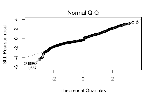
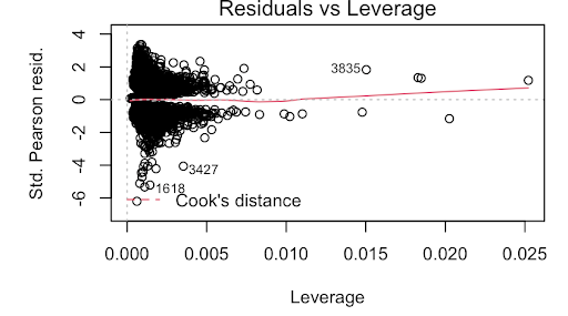
While the predictors in this model were statistically significant and produced a Kaggle Score of 0.8015, this is a very rudimentary model. Thus, we decided to delve deeper into the data to find one that better fit.

Random Forest

We decided to test a Random Forest model since it is an ensemble classifier, one of the most accurate learning algorithms, and runs efficiently on large databases. It also reduces overfit and decorrelates compared to a bagging model which will ultimately lead to a better accuracy; therefore, we attempted to find an optimal Random Forest model.

We used three different Random Forest models: one with all 19 predictors, one with the best 15 predictors, and one with the best 10 predictors. For each of these models, we found the respective mtry value that would produce the lowest misclassification rate.

## Random Forest

library(ggplot2)
library(randomForest)
set.seed(1)
train <- sample(1:nrow(HDtrainMICE.samp.data), round(nrow(HDtrainMICE.samp.data)*.7))

#finding MCRs at different mtry levels for each model
mcr.full <- numeric(19)
for(i in 1:19){
 rf.heart <- randomForest(HeartDisease~., data = HDtrainMICE.samp.data, subset=train, mtry=i,importance = TRUE)
pred.rf<- predict(rf.heart, newdata = HDtrainMICE.samp.data, type = "class")
conf.matrix.rf <- table(pred.rf, HDtrainMICE.samp.data$HeartDisease)
misclass.icu.rf <- (conf.matrix.rf[2,1]+conf.matrix.rf[1,2])/sum(conf.matrix.rf)
 mcr.full[i] <- misclass.icu.rf
}

mcr <- numeric(15)
for(i in 1:15){
 rf.heart.15 <- randomForest(HeartDisease~Oldpeak + avg_glucose_level +MaxHR + Age+Cholesterol+FastingBS +ST_Slope+RestingBP +bmi +ever_married +ExerciseAngina +ChestPainType +smoking_status +Sex + hypertension, data = HDtrainMICE.samp.data, subset=train, mtry=i,importance = TRUE)
pred.rf.15 <- predict(rf.heart.15, newdata = HDtrainMICE.samp.data, type = "class")
conf.matrix.rf.15 <- table(pred.rf.15, HDtrainMICE.samp.data$HeartDisease)
misclass.icu.rf.15 <- (conf.matrix.rf.15[2,1]+conf.matrix.rf.15[1,2])/sum(conf.matrix.rf.15)
 mcr[i] <- misclass.icu.rf.15
}

mcr.10 <- numeric(10)
for(i in 1:10){
 rf.heart.10 <- randomForest(HeartDisease~Oldpeak + avg_glucose_level +MaxHR + Age+FastingBS +ST_Slope+RestingBP +bmi +ChestPainType +smoking_status, data = HDtrainMICE.samp.data, subset=train, mtry=i,importance = TRUE)
pred.rf.10 <- predict(rf.heart.10, newdata = HDtrainMICE.samp.data, type = "class")
conf.matrix.rf.10 <- table(pred.rf.10, HDtrainMICE.samp.data$HeartDisease)
misclass.icu.rf.10 <- (conf.matrix.rf.10[2,1]+conf.matrix.rf.10[1,2])/sum(conf.matrix.rf.10)
 mcr.10[i] <- misclass.icu.rf.10
}

#full model
rf.heart <- randomForest(HeartDisease~., data = HDtrainMICE.samp.data, subset=train, mtry=5,importance = TRUE)
rf.heart
varImpPlot(rf.heart)

#training missclassification rate of full model
pred.rf <- predict(rf.heart, newdata = HDtrainMICE.samp.data[-train,], type = "class")
conf.matrix.rf <- table(pred.rf, HDtrainMICE.samp.data[-train,]$HeartDisease)
misclass.icu.rf <- (conf.matrix.rf[2,1]+conf.matrix.rf[1,2])/sum(conf.matrix.rf)
conf.matrix.rf
misclass.icu.rf #misclassification rate of 0.2014218

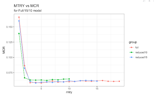
For the full Random Forest model, the best mtry value was 5 so we ran our model with that value. We obtained a misclassification rate of approximately 19.83%. Next, we simplified our model by removing the four worst predictors based on importance. This new 15 predictor model did not include Residence_type, stroke, RestingECG, and work_type. We used a mtry value of 4 since this was the value that created the lowest misclassification rate for this respective model. The misclassification rate was approximately 19.74%, only marginally better than the full model. Finally, we removed the worst five predictors from this model to create our final, 10 predictor model. This model did not have bmi, smoking_status, Sex, ChestPainType, and hypertension. Using a mtry value of 6, the misclassification rate was approximately 21.09% which was the worst of the three models.

#removing the worst 4 for the next model to make model of 15
#worst 4: stroke, residence_type, work_type, and restingECG

rf.heart.15 <- randomForest(HeartDisease~Oldpeak + avg_glucose_level +MaxHR + Age+Cholesterol+FastingBS +ST_Slope+RestingBP +bmi +ever_married +ExerciseAngina +ChestPainType +smoking_status +Sex + hypertension, data = HDtrainMICE.samp.data, subset=train, mtry=4,importance = TRUE)
rf.heart.15
varImpPlot(rf.heart.15)
#worst 5: hypertension, sex, cholesterol, exercise, married

#training misclassification rate of 15 predictor model
pred.rf.15 <- predict(rf.heart.15, newdata = HDtrainMICE.samp.data[-train,], type = "class")
conf.matrix.rf.15 <- table(pred.rf.15, HDtrainMICE.samp.data[-train,]$HeartDisease)
misclass.icu.rf.15 <- (conf.matrix.rf.15[2,1]+conf.matrix.rf.15[1,2])/sum(conf.matrix.rf.15)
conf.matrix.rf.15
misclass.icu.rf.15 #missclassification rate of 0.1999842

#10 predictors
rf.heart.10 <- randomForest(HeartDisease~Oldpeak + avg_glucose_level +MaxHR + Age+FastingBS +ST_Slope+RestingBP +bmi +ChestPainType +smoking_status, data = HDtrainMICE.samp.data, subset=train, mtry=3,importance = TRUE)
rf.heart.10
varImpPlot(rf.heart.10)

#training missclassification rate of 10 predictor model
pred.rf.10 <- predict(rf.heart.10, newdata = HDtrainMICE.samp.data[-train,], type = "class")
conf.matrix.rf.10 <- table(pred.rf.10, HDtrainMICE.samp.data[-train,]$HeartDisease)
misclass.icu.rf.10 <- (conf.matrix.rf.10[2,1]+conf.matrix.rf.10[1,2])/sum(conf.matrix.rf.10)
conf.matrix.rf.10
misclass.icu.rf.10 #missclassification rate of 0.2101106

Compared to our logistic regression with stepwise selection, none of our Random Forest models performed as well. All three models had a higher misclassification error rate. Furthermore, a Random Forest model is rather complex despite our efforts to simplify it and it is much harder to interpret compared to a logistic regression model. Other limitations include the tendency to overfit as well as its bias towards categorical variables with a higher number of levels.

Logistic Regression with Stepwise Selection

For our final model, we decided to run another stepwise logistic regression model, but this time with the categorical and numerical variables selected by the previous stepwise logistic regression models. We ran two models: one with the avg_glucose_level and one with newglucose and their corresponding chosen variables. To decide whether we would use the model with newglucose or avg_glucose_level, we calculated the training misclassification rates of both models and found that the model with avg_glucose_level had a lower misclassification rate (0.1893365 vs 0.1933649). Thus, we decided to use the model with avg_glucose_level and its corresponding chosen variables.

###stepAIC with categorical and numerical variables selected by previous stepAIC models; we will use both the transformed avg_glucose_level (newglucose) and the original avg_glucose_level and their corresponding variables chosen by stepAIC

testing3.step <- stepAIC(glm(HeartDisease ~ Cholesterol+MaxHR+Oldpeak+avg_glucose_level+Sex+FastingBS+RestingECG+ExerciseAngina+ever_married+work_type+Residence_type+stroke, family = binomial, data = HDtrainMICE.samp.data), method = "exhaustive", trace=F)

testing3.step.ng <- stepAIC(glm(HeartDisease ~ Cholesterol+MaxHR+Oldpeak+newglucose+bmi+Sex+FastingBS+RestingECG+ExerciseAngina+ever_married+work_type+Residence_type+stroke, family = binomial, data = HDtrainMICE.samp.data), method = "exhaustive", trace=F)

pred.prob<-predict(testing3.step,type="response",data=HDtrainMICE.samp.data)
predicted.HD<-pred.prob>.5
table(predicted.HD,HDtrainMICE.samp.data$HeartDisease)
(328+471)/4220 #misclassification rate of 0.1893365

pred.prob2<-predict(testing3.step.ng,type="response",data=HDtrainMICE.samp.data)
predicted.HD2<-pred.prob2>.5
table(predicted.HD2,HDtrainMICE.samp.data$HeartDisease)
(339+477)/4220 #misclassification rate of  0.1933649, which is higher than that of testing3.step, so we will use the model with the original avg_glucose_level

In the end, we decided to choose this as our final model, as it was the simplest model with the smallest training misclassification rate. It scored 0.80869 on Kaggle, which is our best score.

###Final Model Selection
**We chose the model that had both the smallest misclassification rate and was the simplest: our stepAIC (stepwise selection using forward and backwards selection) model with logistic regression using the original avg_glucose_level and other variables chosen by stepAIC**

pred.prob10 = predict(testing3.step,type="response",data=HDtrainMICE.samp.data, newdata = HDtestMICE.samp.data)

D.glm.pred10=rep("No",dim(HDtestMICE.samp.data)[1])
D.glm.pred10[pred.prob10>0.5]="Yes"

HDtest.pred10 <- as.data.frame(D.glm.pred10)
HDtest.pred10[,2] = HDtest.pred10[,1]
HDtest.pred10[,1] = 1:1808
colnames(HDtest.pred10) <- c("Ob", "HeartDisease")

write.csv(HDtest.pred10, "/Users/k/Documents/STATS 101C/Data sets/test10.pred.csv", row.names = FALSE)

#scored 0.80869 on Kaggle

Conclusions and Limitations

Conclusions

In conclusion, our stepwise logistic regression model outperformed the other logistic regression and random forest methods in classifying or predicting Heart Disease. This model had a misclassification rate of 0.1893365, with a score of 0.80869 on Kaggle. When building and fine-tuning this model, the missing data points were imputed by comparing the performance of different methods in the MICE package. Furthermore, the numerical and categorical variables used were chosen based on a combination of techniques, including both forward and backward stepwise selection. Due to the fact that machine learning models have the potential to significantly improve the accessibility of accurate and timely heart disease diagnoses, this project has substantial importance in the real world. Catching or predicting the disease early on is crucial to saving patients; therefore, further research and analysis of utilizing machine learning methods to predict heart disease is very important. In fact, while this project allowed us to explore how to improve the accuracy of diagnoses using data mining, it included variables that may be inaccessible to many people (ex. ECG tests). Thus, for further research, it’s important to consider the idea of building models with high accuracy using only basic predictors, such as Sex, age, etc (Gavhane A. et al.).

Limitations

While we believe our model’s performance was satisfactory, our analysis still has some limitations. The first limitation of our model is that outliers in the numerical predictors Cholesterol, OldPeak, and avg_glucose_level may make our model more inaccurate. One other possible limitation is that the methods used to impute the missing values may have produced wrong observations leading to a less accurate model. Another possible limitation of our analysis is that there may be much more valuable variables that could be used to predict heart disease that weren’t included in the data set or used in the analysis.

References

Abdar M, Książek W, Acharya UR, Tan RS, Makarenkov V, Pławiak P. A new machine learning technique for an accurate diagnosis of coronary artery disease. Comput Methods Prog Biomed. 2019;179:104992.

Dai W, Brisimi TS, Adams WG, Mela T, Saligrama V, Paschalidis IC. Prediction of hospitalization due to heart diseases by supervised learning methods. Int J Med Inform. 2015;84(3):189–97.

Gavhane A. “Prediction of Heart Disease Using Machine Learning” Second International Conference on Electronics, Communication and Aerospace Technology (ICECA), (Iceca); 2018. p. 1275–8.

Khourdifi Y, Bahaj M. Heart Disease Prediction and Classification Using Machine Learning Algorithms Optimized by Particle Swarm Optimization and Ant Colony Optimization. Int J Intell Eng Syst. 2019;12(1):242–52. https://doi.org/10.22266/ijies2019.0228.24.

Krishnaiah V, Chandra NS. Heart disease prediction system using data mining techniques and intelligent fuzzy approach: a review. Int J Comput Appl. 2016;136(2):43–51.